University of Connecticut Active Collimator Station Tutorial
On January 7th, 2014, the active collimator station (computer name actcol-station) was positioned in room F117 of the CEBAF building at Jefferson Lab. This wiki page serves to teach how the station operates.
Configuration of the station
Figures 1 and 2 serve to show the user how the active collimator station is connected to the actcol-station PC. I have labeled various components in Figure 1; their descriptions are below. Figure 2 shows the user how to connect everything to the PC. Figure 3 is used later in the tutorial.
(1 and 2) Collimator and amplifiers: The signals from the tungsten plates within the active collimator are picked up and transmitted to the amplifiers via an SMA to BNC cable.
(3) Amplifier signal output and power/range input: On the "downstream" end of the amplifiers, there is a connection for a BNC to BNC cable that is used to transmit the amplified signals to the BNC box (5). There is also a DB9 to Ethernet adapter; connecting an Ethernet cable from the Ethernet splitter (4) supplies power and information from the terminal board (6).
(4) Ethernet "splitter": This is for power distribution and communication with the terminal board (6). From right to left: power source from F100-PS power supply (not pictured), four power sources for the amplifiers, connection to terminal board.
(5) "BNC Box": A BNC to BNC cable connects each amplifier to the BNC box. The BNC box is then connected to the terminal board (6) and PC via a ribbon cable. Connect the end of the ribbon cable labeled "BNC box" to the "P3" input in the back of the BNC box.
(6) Terminal board: Connect the end of the ribbon cable labeled "terminal board" to the (you guessed it) terminal board. See Figure 2 for a better view.
Connect the remaining end of the ribbon cable to the data acquisition card in the PC. The gain setting for the amplifiers is chosen within the LabVIEW program, which is discussed next.
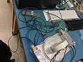
Figure 1
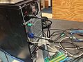
Figure 2
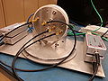
Figure 3


The actcol-station should always be running. Before running the program, be sure to change the rocker switch on the back of the F100-PS power supply to the "on" position!
Igor Senderovich, a former PhD student who worked under the supervision of Dr. Richard Jones, wrote a LabVIEW program that contains many useful features for acquisition and analysis of signals from the active collimator. This program can be accessed on the actcol-station (you may need the Student user account password in order to access it; email the address at the bottom of this wiki page with a request).
In order to start the program, click the "Shortcut to MCChannelScanEnhanced_4-chan(current)" icon on the desktop, indicated by the green arrow below. A window will open; choose MCChannelScanEnhanced_4-chan(current).vi, indicated by the red arrow.

Once the program opens, press the "Run" arrow.

The LabVIEW program is now active. Choose Board Num 0. NChan is the number of channels you want LabVIEW to take data from; in this case, there are 4 channels. You can also choose specific channels from the BNC box with Ch1. The Range option tells LabVIEW the range (plus and minus) in which it measures exact potential differences. The time window(s) option tells the program how long to take data within each Interval(s); there is also an overhead selection. (In LabVIEW, "100m" means 100 milliseconds.) The Gain setting drop-down window allows the user to choose the gain setting for the amplifiers in powers of ten from 10^6 to 10^12. Make sure you click "set" before acquiring data! The Averages drop-down menu averages the signal; this is useful for beam data acquisition. The Trigger box works the same as an oscilloscope; you can manipulate the trigger position above the signal displays (the four black boxes with green grids on the left). The Min and Max settings next to the signal displays change the user's signal view, but does not alter the data acquisition process. The lower left section of the program is only used when the collimator is installed in the "Collimator cave;" I was told this program will no longer be used upon its future installation. The top right black window with green grid is a display of a fast Fourier transform for a selected channel. This feature can be turned on by pushing the button next to "FT;" more on this later. I have never used the bottom right black window with green grid. The picture below depicts the settings I used before running the program.

You now must choose where you would like a History file to be saved; this also sets the destination for the acquired waveforms. Choose Set History File on the bottom right of the program to choose its destination and to name it. For the purposes of this tutorial, I chose the History File name to be "Test" and made a folder named "Test" on the desktop to save the waveforms to. Next, check the "Record History" box. Then check the "Save Waveforms" box. You can input the "file prefix" for the acquired waveforms; the default is "trc_."

You can now click Run on the top right. With the options selected in this tutorial, all four signal displays will refresh every second. The picture below depicts the LabVIEW program acquiring data and performing a Fourier transform on Channel 0 (the leftmost tungsten wedge, according to the orientation in Figure 3 at the top of this wiki page). The other Fourier transform options are self-explanatory.

There are visible brass screws on the face plate of the active collimator (Figure 3). Each of these screws are connected to a separate tungsten plate. Touching these screws with a piece of metal that is in contact with your hand will send electrons into the plates. This reaction is very obvious when looking at the signal displays. To record a useful waveform, you must tap one of the screws very lightly and quickly. You may also hold the piece of metal on the screw to become a human antenna! I should mention that the best waveforms are acquired at very high gain settings. Click Run once more to terminate the program. You have now acquired data from the active collimator!
The History file contains the following information by column: acquisition number (matches trace file numbering), absolute acquisition time (sec), collimator x-displacement (in), beam current (nA), and the four plate signals (V).

The waveform files contain the following information by column: timestamp (sec) and the four plate signals (V).

Installation of additional tungsten plates
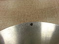
Circle

UNDER CONSTRUCTION
Feel free to contact me at john DOT bartolotta AT uconn DOT edu with any questions.