Difference between revisions of "Offline Monitoring Data Validation CPP"
(→FDC) |
(→FDC) |
||
| Line 281: | Line 281: | ||
<html> | <html> | ||
| − | There are two HV sectors, in Package 2 cell 6 and Package 3 cell 4, that are always OFF and seen in the occupancy plots as | + | There are two HV sectors, in Package 2 cell 6 (28 wires) and Package 3 cell 4 (20 wires), that are always OFF and seen in the occupancy plots as empty sectors. There are also strips with lower or no efficiency that are always there, mostly in Package 3 and 4 (see the reference plots), which also normal. |
| + | What is not normal are groups of wires (of the order of 8 to 24 wires) that are noisy. They will show as brighter stripes in the occupancy. The problem is that they may lock the F1TDCs. This happened several times in the past years. In general, look for groups of channels that are overactive or have lower efficiency. | ||
| + | \ | ||
</html> | </html> | ||
Revision as of 01:20, 30 November 2023
This page contains the procedure for checking if CPP/NPP production runs are of good quality and can be used for physics analysis.
Contents
Procedure
For each production run, do the following:
- Go to the Offline Plot Browser page.
- Make sure that you are looking at the correct monitoring version (currently ver23).
- Follow the steps outlined in the checklist below.
- Workers should check each plot for their assigned subsystem and leave notes in the corresponding spreadsheet if any significant deviations are seen
- On the spreadsheet page for the relevant subsystem, enter "Y" in the "Overall Quality" field if all monitoring histograms are acceptable, otherwise enter "N"
- We will iterate this procedure until the process converges
Expert Actions
- Certify that each subsystem is okay
- Set run status in RCDB based on monitoring results
- (script provided)
Run Statuses
- -1 - unchecked
- 0 - rejected (not physics-quality)
- 1 - approved
- 2 - approved long/"mode 8" data
- 3 - calibration / systematic studies
Checklist
Reference run for 2022-05: 100987
Instructions Status and Responsible Parties
- Ready:
- CDC: Naomi Jarvis
- PS: Experts: Alex Somov, Olga Cortes. Instructions from Sean Dobbs
- TAGH: Experts: Alex Somov, Bo Yu. Instructions from Sean Dobbs
- TAGM: Experts: Richard Jones, Ellie Prather. Instructions from Sean Dobbs
- TOF: Beni Zihlmann
- Ready after new monitoring launch:
- Timing: Sean Dobbs
- In progress:
- BCAL: Mark Dalton, Zisis Papandreou
- CTOF: Albert Fabrizi
- FCAL: Mark Dalton, Malte Albrecht
- FDC: Lubomir Pentchev
- FMWPC: Albert Fabrizi
- Analysis: Alex Austregesilo
Monitoring Volunteers
- Ready to start:
- CDC: Alison Laduke
- PS: Ahmed Foda
- TAGH: Saheli Rakshit
- TAGM: Saheli Rakshit
- TOF: Jesse Hernandez
- Standby:
- BCAL: Zisis Papandreou/Regina + Tolga Erbora
- CTOF: Albert Fabrizi
- FCAL: Ahmed Foda
- FDC: Dene Hoffman
- FMWPC: Albert Fabrizi
- Timing: Nizar Septian
- Analysis: Zach Baldwin
General Notes
- Diamond and amorphous (AMO) runs have different beam energy spectra, which leads differences in reaction yields distributions which depend on the kinematics of the produced particles.
- The list of experts on different detector/calibration
BCAL
- Check Occupancy - Reference: [ link ]
- Check Hit Efficiency - Reference: [ link ]
- Check Recon. BCAL 1 - Reference: [ link ]
- Check Recon. BCAL 2 - Reference: [ link ]
- Check BCAL Matching - Reference: [ link ]
BCAL Reference Plots


BCAL Notes
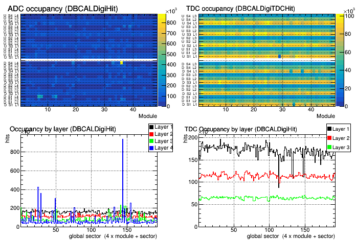
The BCAL is used to measure the energy and time of showers.
- Occupancy: This should be approximately flat. There can be hot channels when the baseline drifts. If we're running ask for a pedestal calibration to be done. If we're not running nothing can be done but a very hot channel might explain low efficiency in that area.
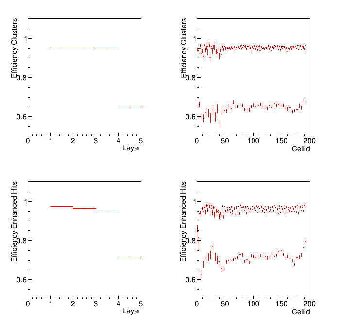
- Hit Efficiency: This should be approximately flat. If there are features we should understand why.
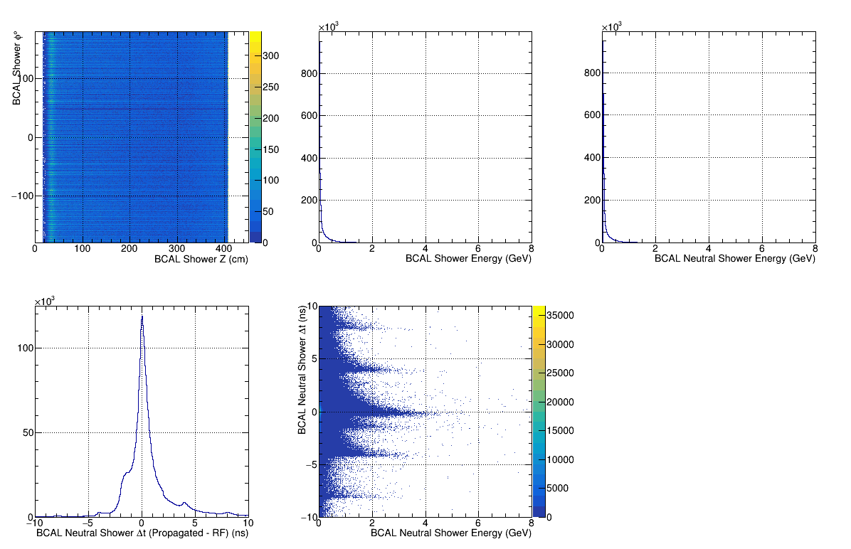
- Recon. BCAL 1: The histograms are somewhat complicated. The best is to compare them to a good run (the example above.) A difference from the example should be flagged.
- Recon. BCAL 2: The histograms are somewhat complicated. The best is to compare them to a good run (the example above.) A difference from the example should be flagged.
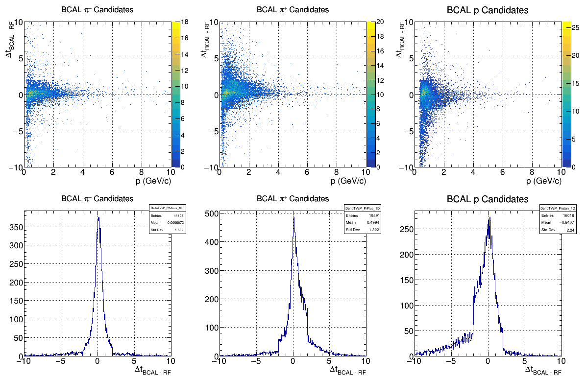
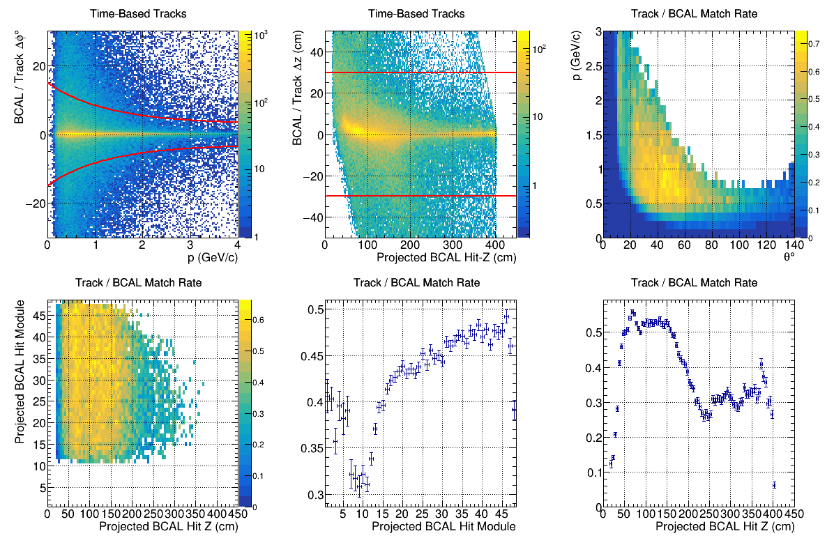
- BCAL Matching: These plots are for charged particles that are tracked in the drift chambers and projected to the BCAL. The z position along the BCAL can be calculated using the time difference between upstream and downstream hits and compared to the extrapolated position using the drift chambers. The histograms are somewhat complicated. The best is to compare them to a good run (the example above.) A difference from the example should be flagged.
- BCAL / Track Delta z (cm): (z determined from time of up - down hits in BCAL) - (z determined from the extrapolation of tracks in the drift chambers)
- projected BCAL Hit-Z (cm): z determined by extrapolating tracks in the drift chambers to the BCAL.
- Track / BCAL Match Rate: The match rate is the ratio of (number of hits in the BCAL that match the extrapolation of tracks in the drift chamber) / (number of tracks in the drift chamber that point at the BCAL).
CDC
- Check Occupancy - Reference: [ link ]
- Check Time-to-distance - Reference: [ link ]
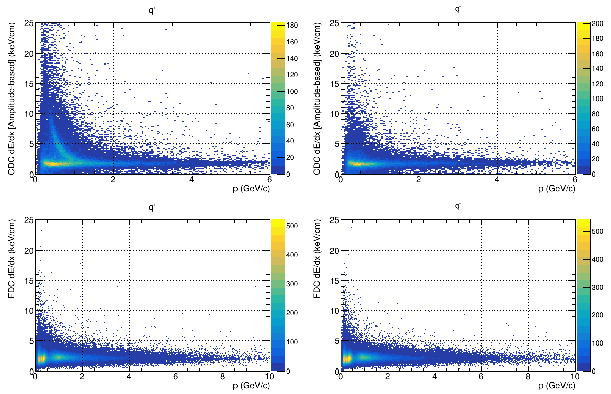
- Check dE/dx - Reference: [ link ]
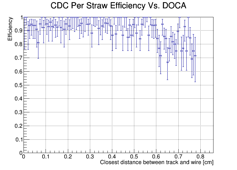
- Check Efficiency- Reference: [ link ]
CDC Reference Plots

CDC Notes
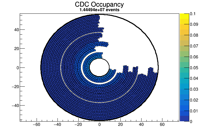
General note: The electronics for the top right quadrant of the detector were borrowed, and used for the muon chambers. The forward trigger configuration did not favour the CDC and its plots from CPP suffer from much fewer statistics than GlueX or PrimEx. It is not a critical detector for this experiment and because of the difficulty of calibrating the data, the usual requirements were relaxed. Many of the runs don't have enough statistics to evaluate them properly. If the run is not definitely bad, then please mark it as good.
CDC Occupancy: It hurts me to look at these plots. For the remaining 3/4 of the detector, there should be a uniform decrease in intensity from the center of the detector outward. Random white cells scattered throughout occur when not enough data were collected, eg empty target runs, trigger tests or no beam. Several contiguous white, dark blue or bright yellow cells which don't match the neighboring cells are a problem.
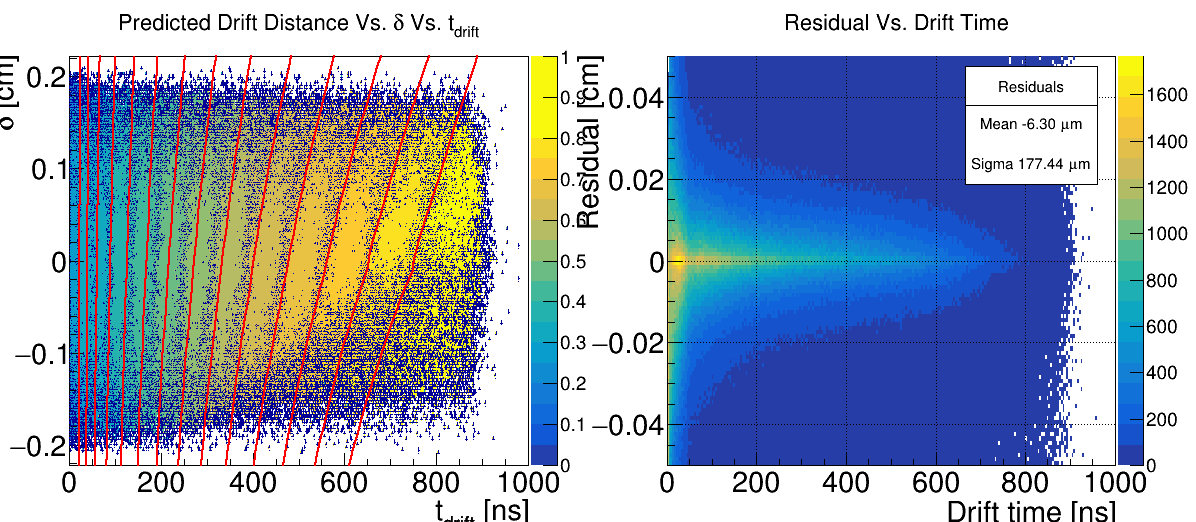
Time-to-distance: 𝛿, the change in length of the LOCA caused by the straw deformation, is
plotted against the measured drift time, t drift. The color scale indicates the distance of
closest approach between the track and the wire, obtained from the tracking software.
The red lines are contours of the time-to-distance function for constant drift distances
from 1.5 mm to 8 mm, in steps of 0.5 mm. They should lie over the top of the dark blue contour lines separating the colour blocks.
For the plot of residuals vs drift time, the mean should be less than 20um and the sigma should be less than 200um.
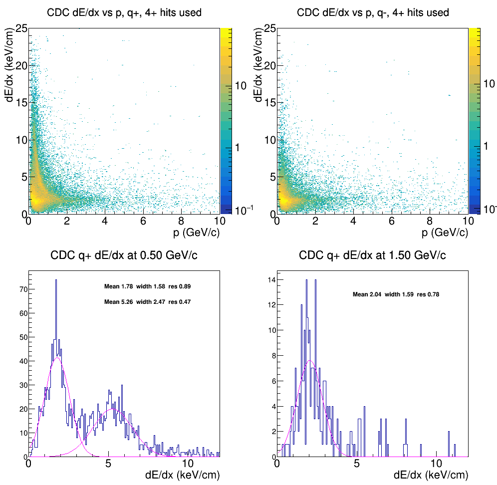
dE/dx: At 1.5GeV/c the fitted peak mean should be within 10% of 2.02 keV/cm.
Efficiency: The efficiency should be 0.9 or higher at 0 to 0.5cm and then fall to around 0.6 or above at 0.75cm.
CTOF
CTOF Reference Plots
CTOF Notes
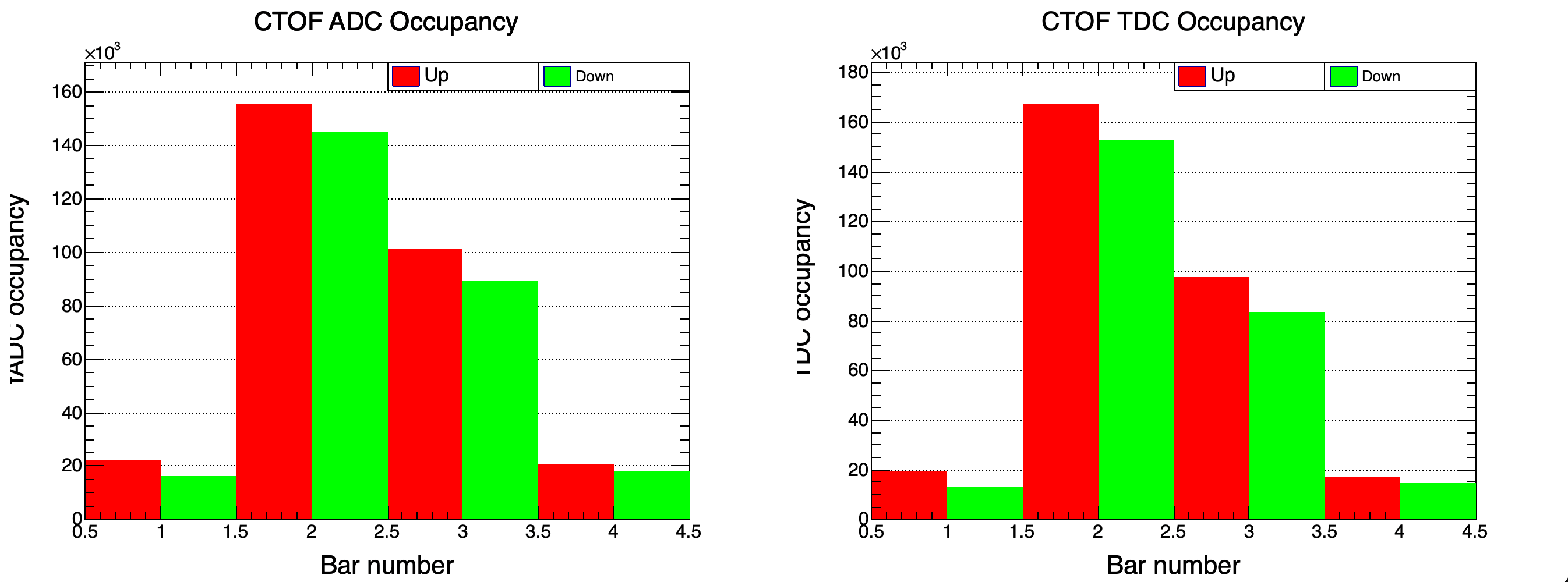
Occupancy: Should show bars 2 and 3 for both ADC and TDC have magnitudes higher more hits than 1 and 4 (2 and 3 are closer to beam line). Occupancy for digi hits only!
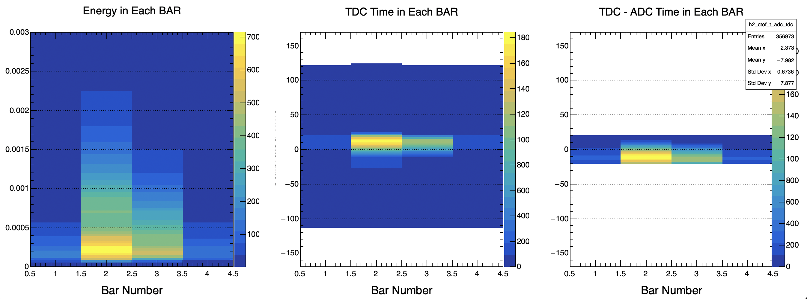
Timing: TDC timing should have a hot peak centered close to zero, with a flat pedestal. The difference in ADC and TDC time should also show a distribution centered close to zero. These are all Calibrated hits.
Pulse Integral: Pulse integral values have a large peak very close to zero relative to the rest of the distribution.
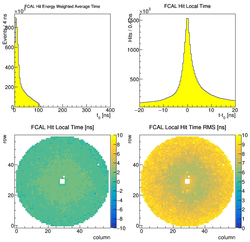
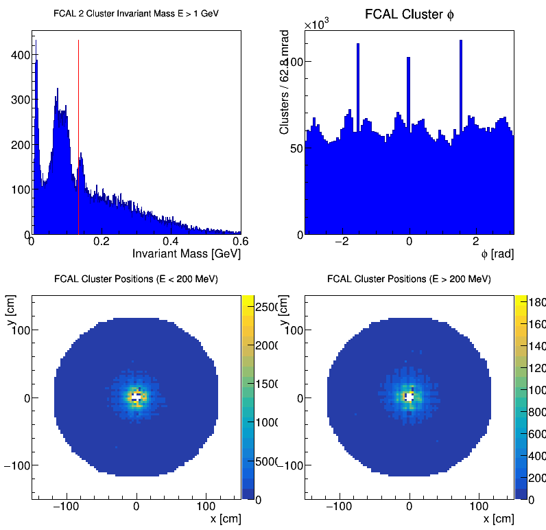
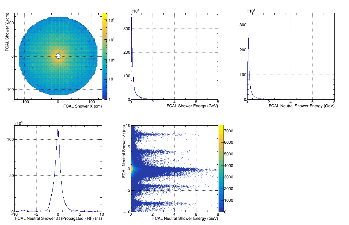
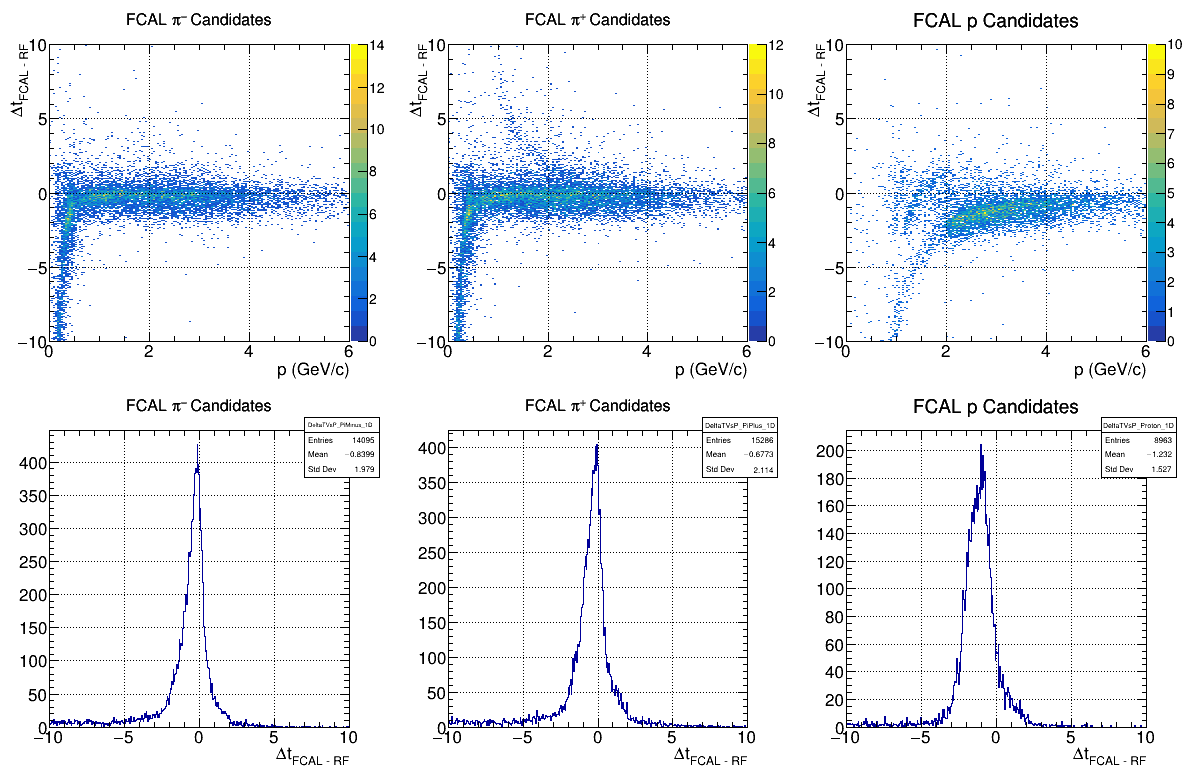
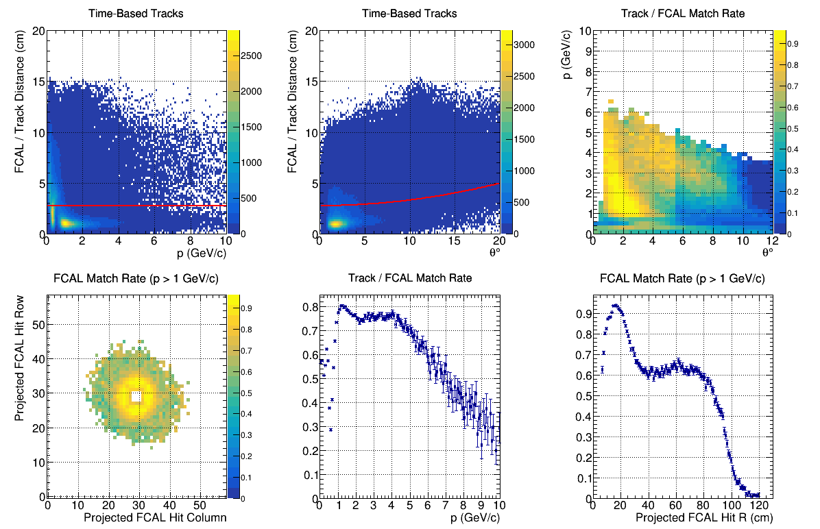
FCAL
- Check Occupancy - Reference: [ link ]
- Check FCAL Hits 1 - Reference: [ link ]
- Check FCAL Hits 2 - Reference: [ link ]
- Check FCAL Clusters 1 - Reference: [ link ]
- Check FCAL Recon. 1 - Reference: [ link ]
- Check FCAL Recon. 2 - Reference: [ link ]
- Check Recon. FCAL Matching - Reference: [ link ]
FCAL Reference Plots
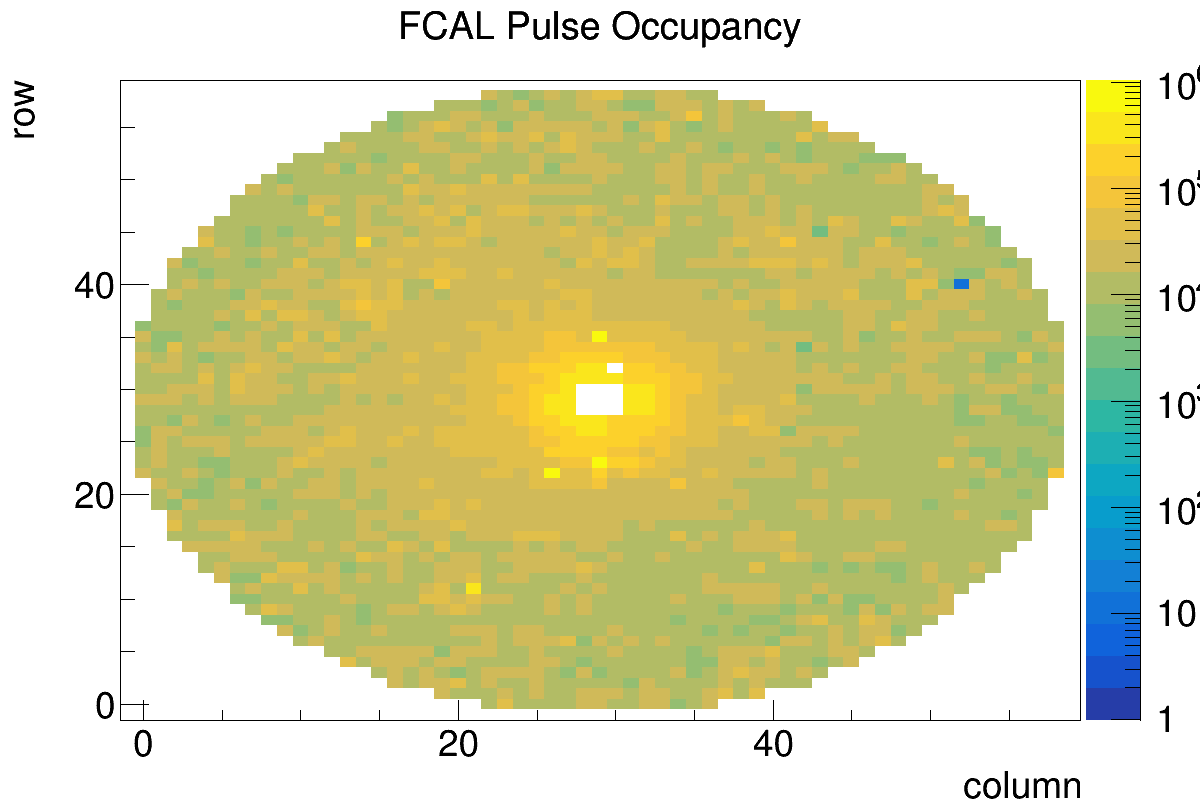


FCAL Notes
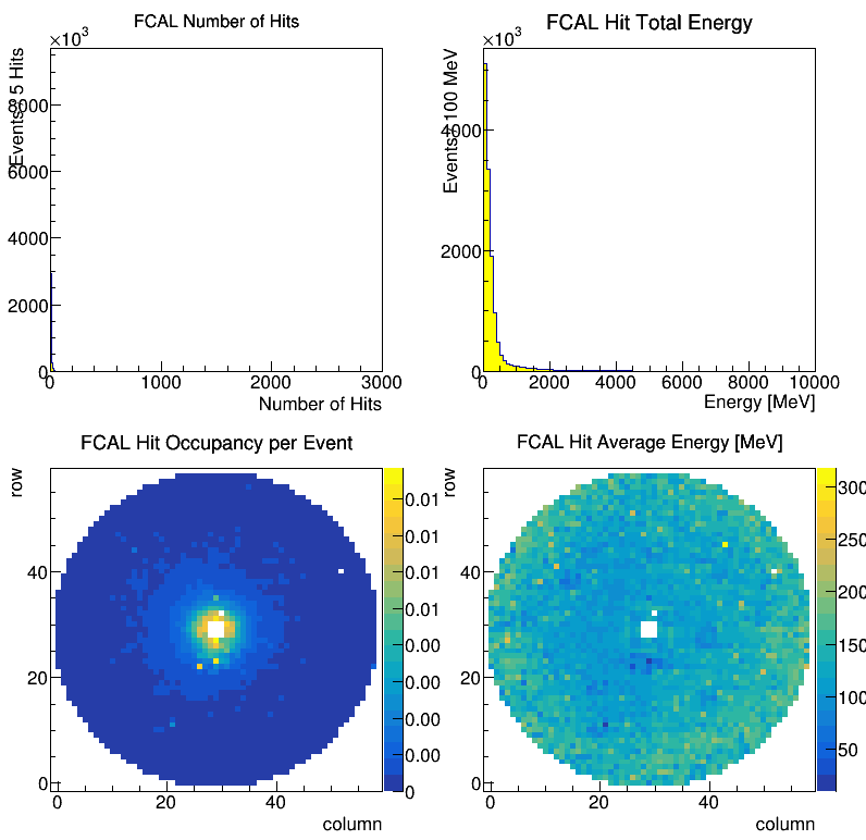
Is used for neutral particle detection and pion identification.
- Check Occupancy:
- Check FCAL Hits 1:
- Check FCAL Hits 2:
- Check FCAL Clusters 1:
- Check FCAL Recon. 1:
- Check FCAL Recon. 2:
- Check Recon. FCAL Matching:
FDC
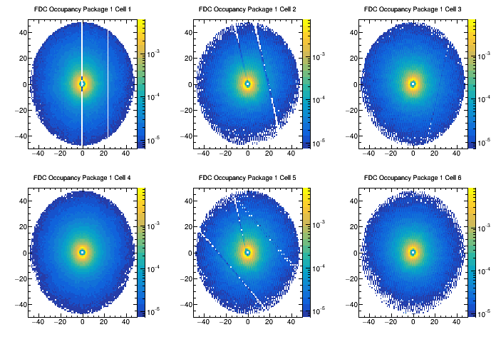
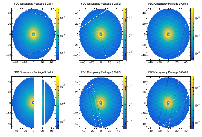
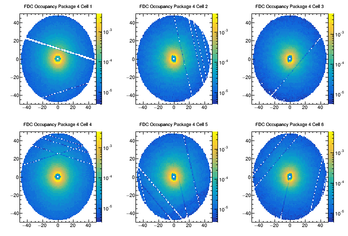
- Check Package 1 Occupancy - Reference: [ link ]
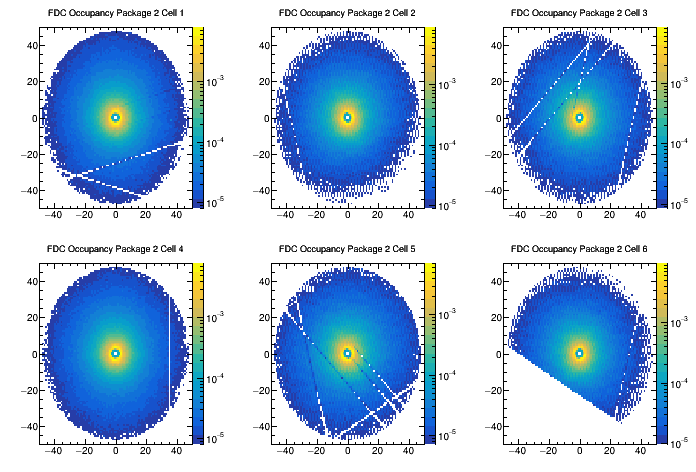
- Check Package 2 Occupancy - Reference: [ link ]
- Check Package 3 Occupancy - Reference: [ link ]
- Check Package 4 Occupancy - Reference: [ link ]
FDC Reference Plots


FDC Notes
There are two HV sectors, in Package 2 cell 6 (28 wires) and Package 3 cell 4 (20 wires), that are always OFF and seen in the occupancy plots as empty sectors. There are also strips with lower or no efficiency that are always there, mostly in Package 3 and 4 (see the reference plots), which also normal. What is not normal are groups of wires (of the order of 8 to 24 wires) that are noisy. They will show as brighter stripes in the occupancy. The problem is that they may lock the F1TDCs. This happened several times in the past years. In general, look for groups of channels that are overactive or have lower efficiency. \
FMWPC
FMWPC Reference Plots
FMWPC Notes
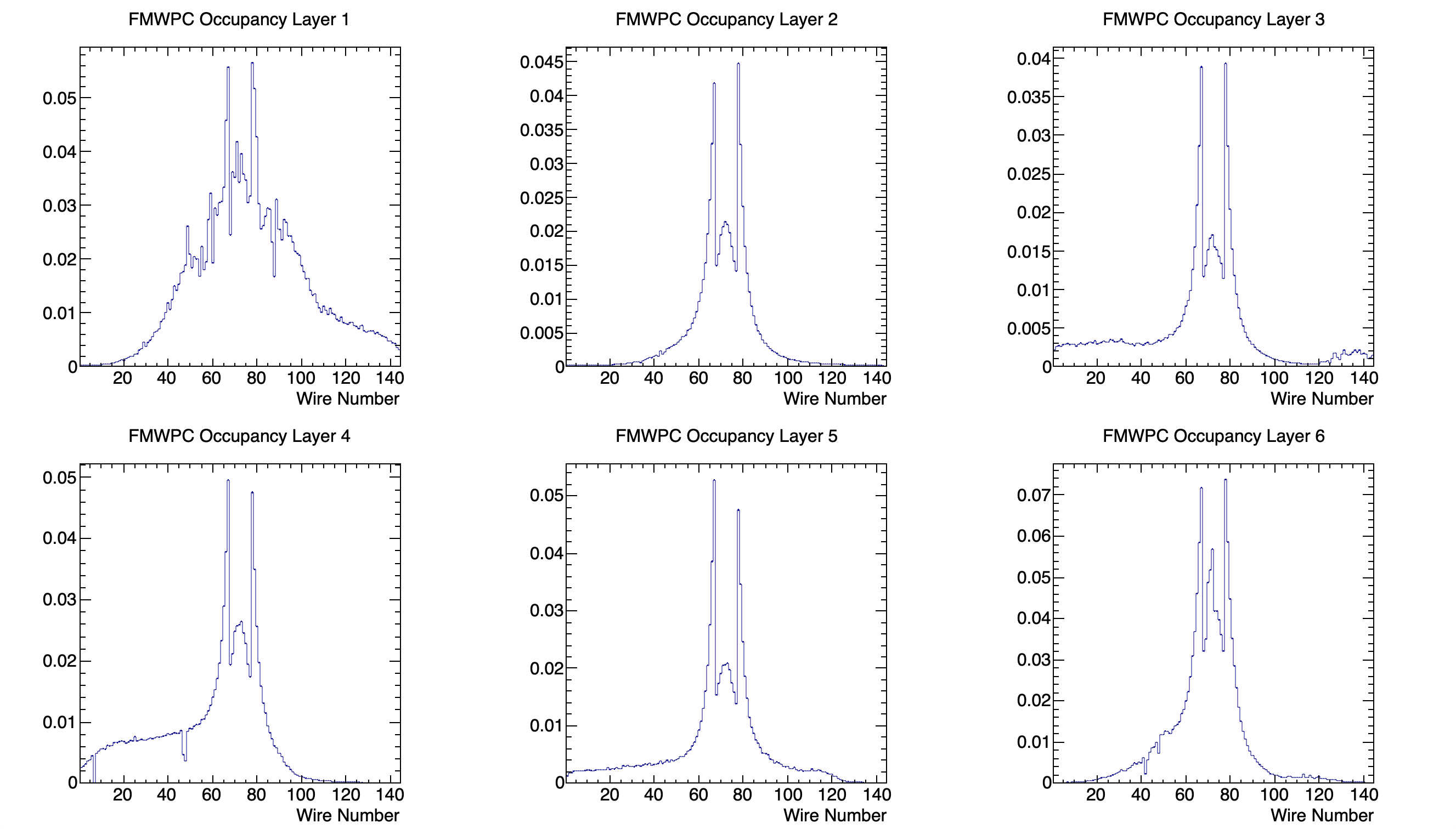
Occupancy: This should show a double peak structure located at the wires close to the beam line and a steady decrease in hits as the wire number gets further from beam line.
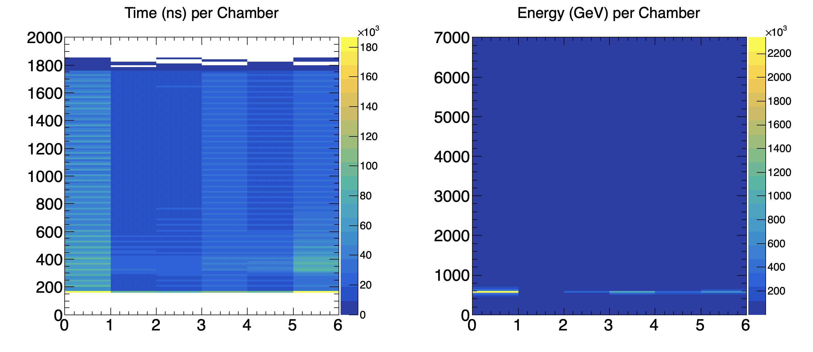
Timing: Shows many small peaks over the whole distribution per chamber. Timing configuration and calibration may have to be done to actually analyze the data from these plots. For now the digi hits can be used for monitoring but the factory (calibrated) hits should be used for analysis until these timing plots are better understood.
Pulse Integral: Should show hot zone around 600, with a flat distribution for the remainder of the range.
PS
PS Reference Plots
PS Notes
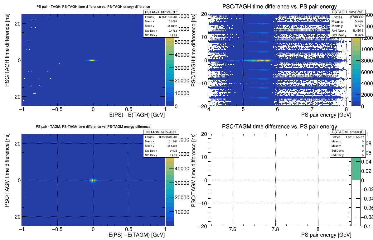
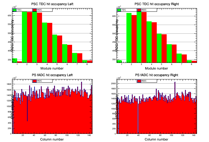
PS Occupancy: PS Occupancy (bottom) should be fairly flat with a couple bad channels. PSC Occupancy (top) should have similar rates in TDC and ADC, with the same shape as the reference histogram. PS Timing: All plots should be centered at zero. The right column reflect the tagger energy, the bottom right is empty (should be updated?).
TAGH
TAGH Reference Plots

TAGH Notes
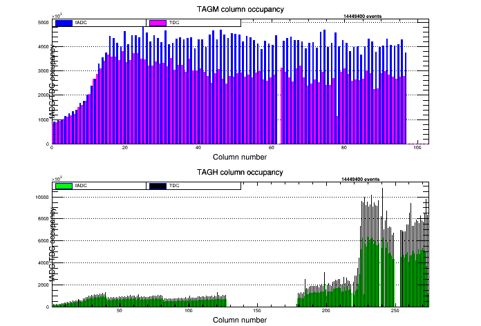
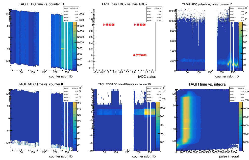
Tagger occupancy: TAGH - Generally the fADC and TDC occupancies should be similar and mostly flat, except for a drop near the left hand side, which represents the location of the coherent peak. TAGH - expect the choppy pattern in the reference image, which reflects the varying size of the different counters
TAGH Hits 2: This plot is complicated - the main thing to look for is the time(TDC)-time(ADC) vs. channel plot to be centered around zero. Keep an eye out for any extra or unusual dead channels.
TAGM
TAGM Reference Plots
TAGM Notes
Generally both distributions should be centered near zero. There is some variation in intensity due to the shape of the photon beam energy dependence (coherent peak) and the inefficiency of some of the channels.
TOF
TOF Reference Plots
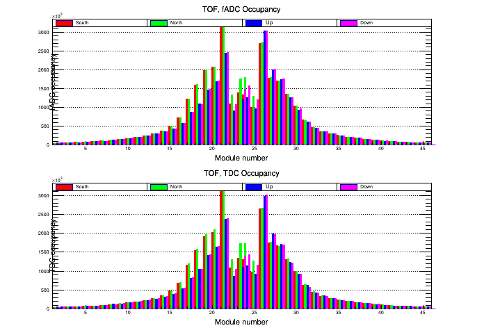
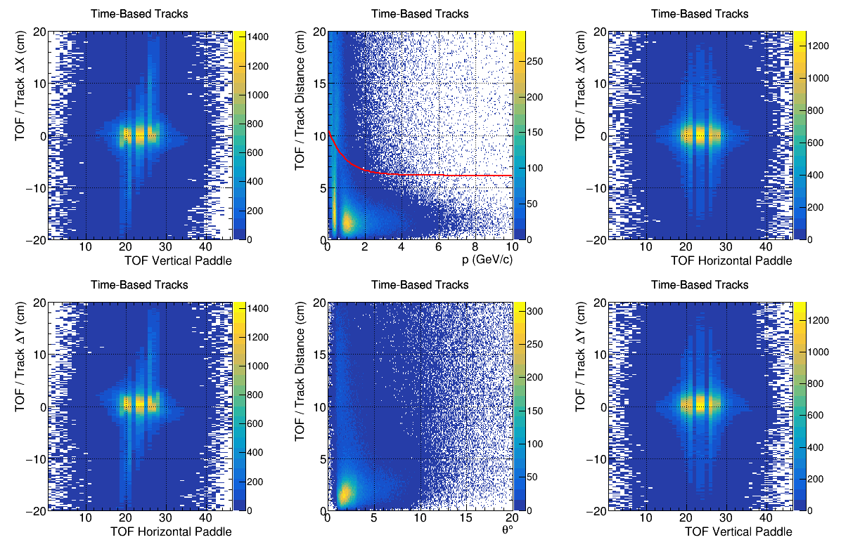
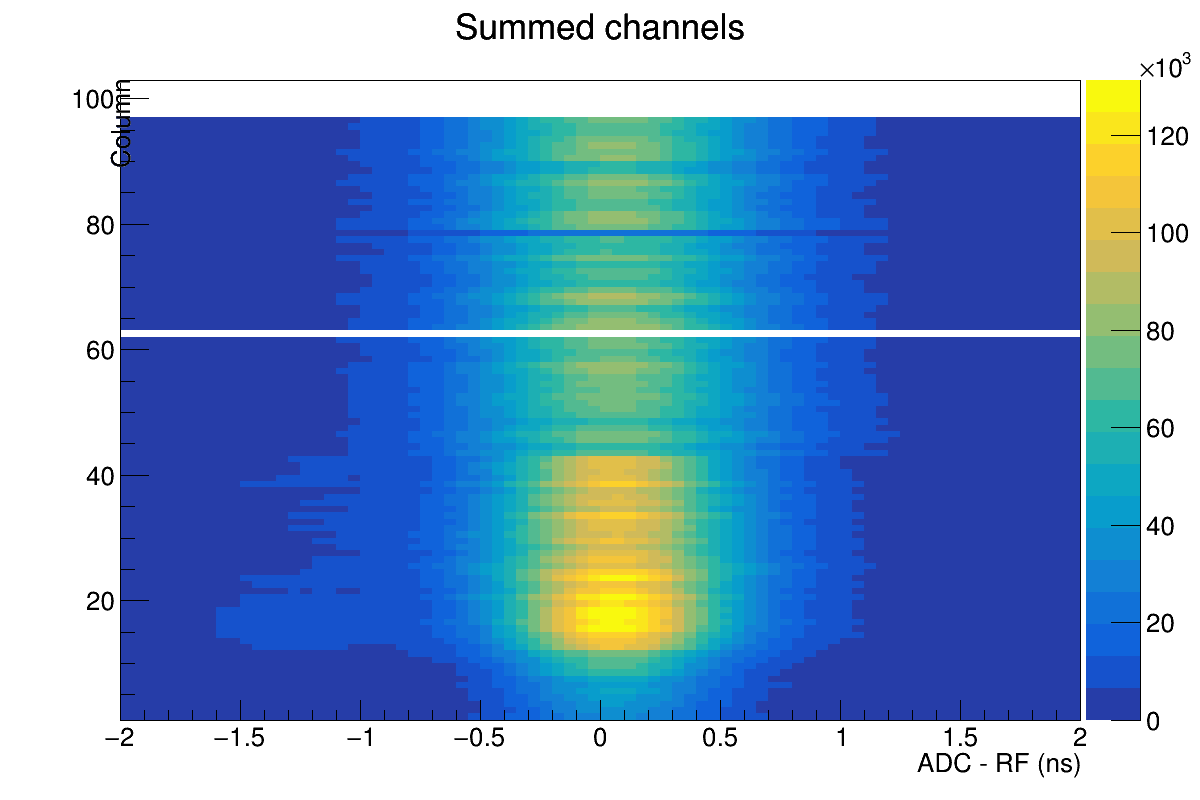
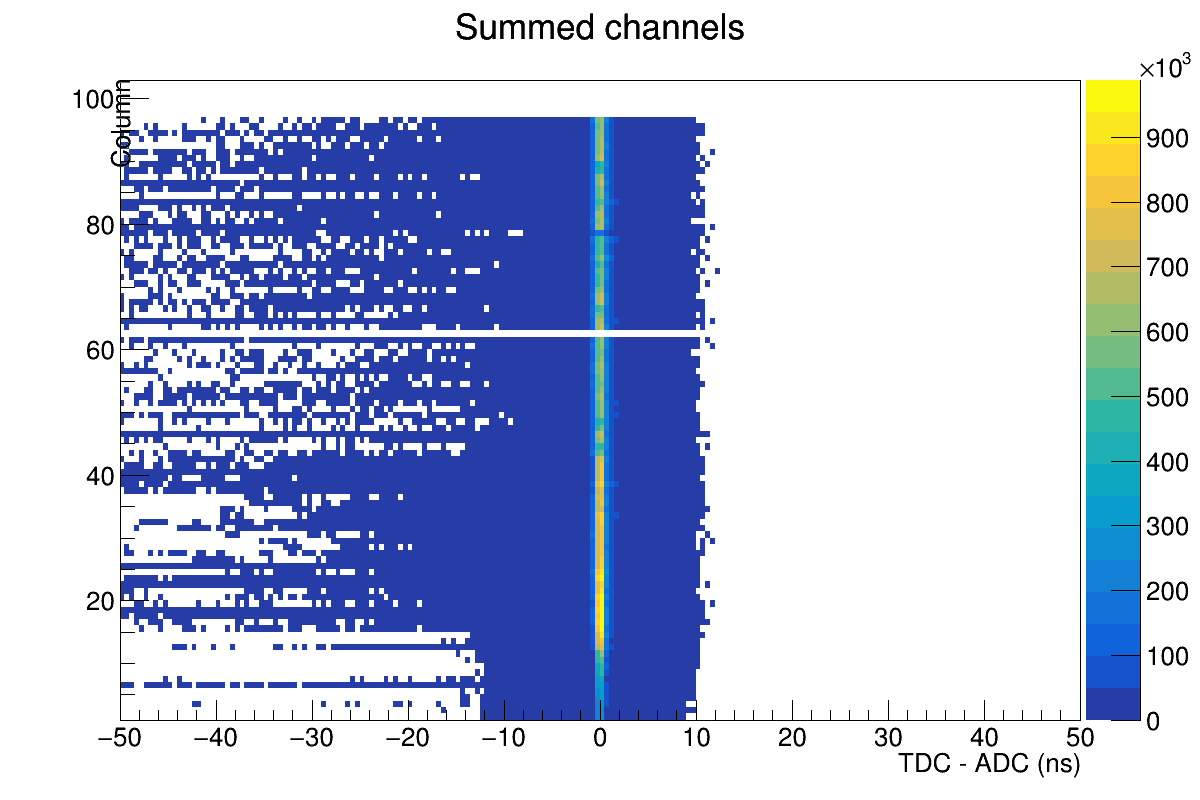
TOF Notes
- Occupancy plot: missing paddles would appear as "gaps" and indicate most likely HV loss.
- Time-Based Tracks: matching of track position at TOF location in x of horizontal paddles and y for vertical paddles, in the third column of he picture, all paddles(x-axis-bins) should have their intensity centered close to zero. This is indicative of a good timing calibration of each paddle/PMT.
Timing
- Check HLDT Calorimeter Timing - Reference: [ link ]
- Check HLDT Drift Chamber Timing - Reference: [ link ]
- Check HLDT PID System Timing - Reference: [ link ]
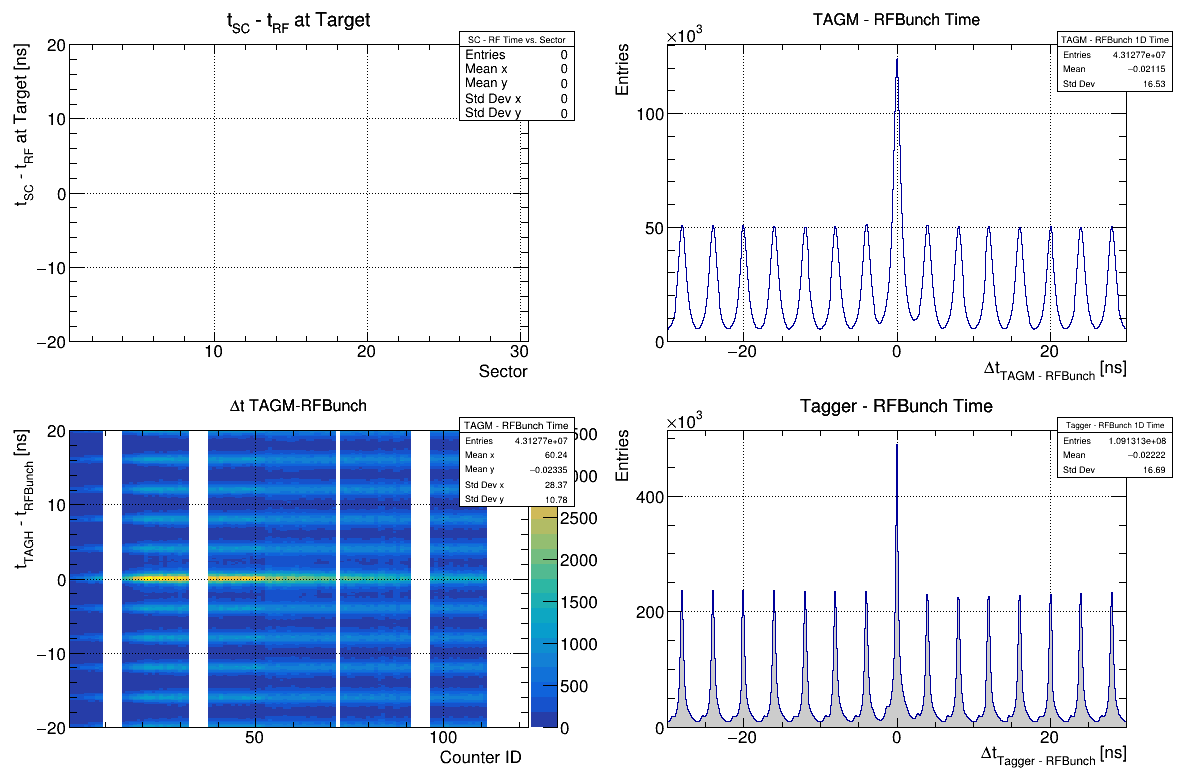
- Check HLDT Tagger Timing - Reference: [ link ]
- Check HLDT Tagger/RF Align 2 - Reference: [ link ]
Timing Reference Plots

![]()

Timing Notes
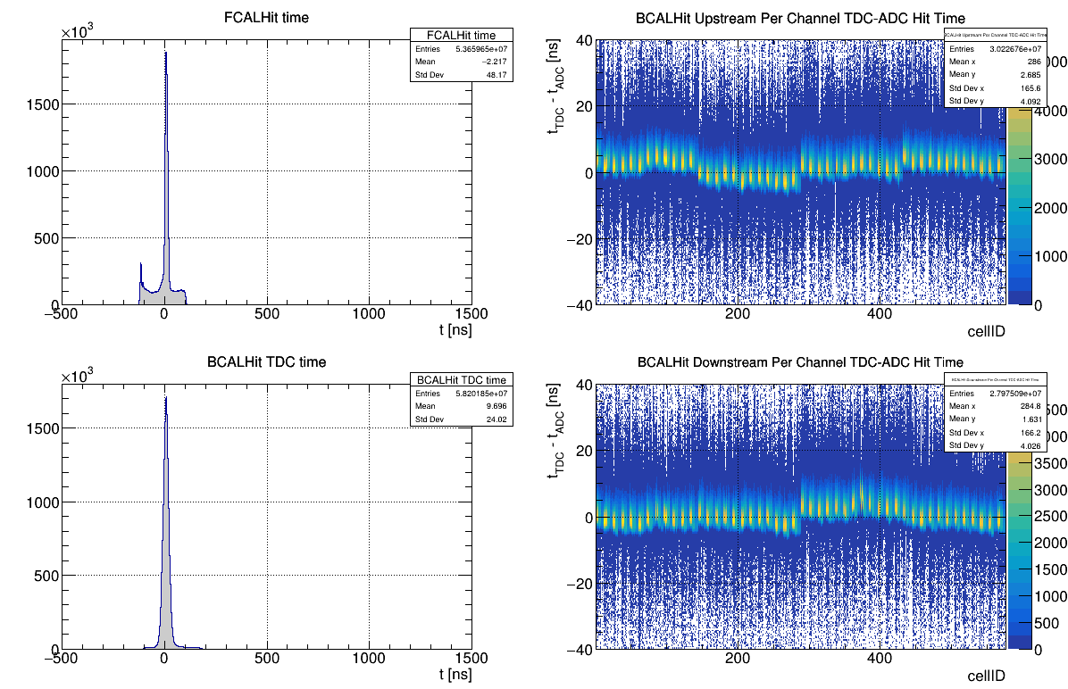
- Calorimeter Timing - Generally the left two peaks should be aligned near zero. The pattern in the right two plots should look like the reference.
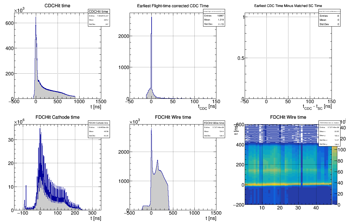
- Drift Chamber Timing - In each case, the main peaks should line up at zero, but often have other structures. Ignore the first few bins of the lower left plot (they mostly say something about the noise in the detector). The signal / noise ratio (main peak vs. other) can change for empty target runs
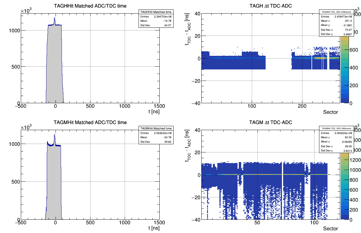
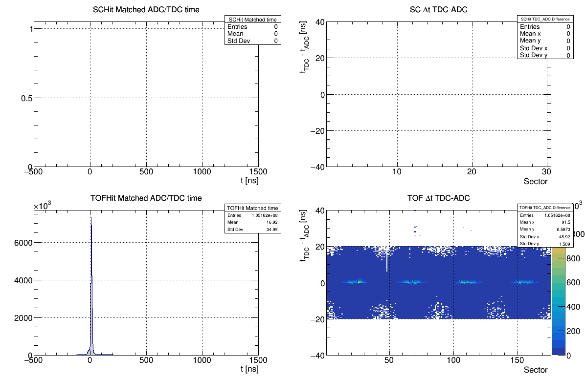
- PID System Timing - The TOF peaks should be near zero. The pattern in the TDC-ADC plot reflect the different occupancies. The SC plots are empty since it was not installed this run.
- Tagger Timing - The signal to background levels of the left two plots depend on the electron beam current. Look for clean peaks in the left two plots, with well-defined edges of the distribution. The right two plots should peak near zero - the blank spots are due to channels that are dead or not installed, and the variation in intensity mostly reflects the photon beam intensity.
- Tagger/RF Timing - Look for the nice "picket fences" on the right two plots, and that in the bottom left plot each channel peaks at zero.
Analysis
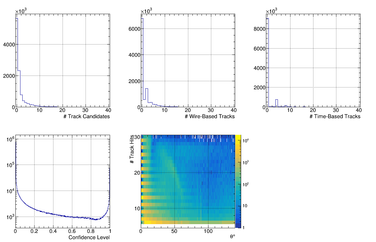
- Tracking 1 - [ link ]
- Tracking 3 - [ link ]
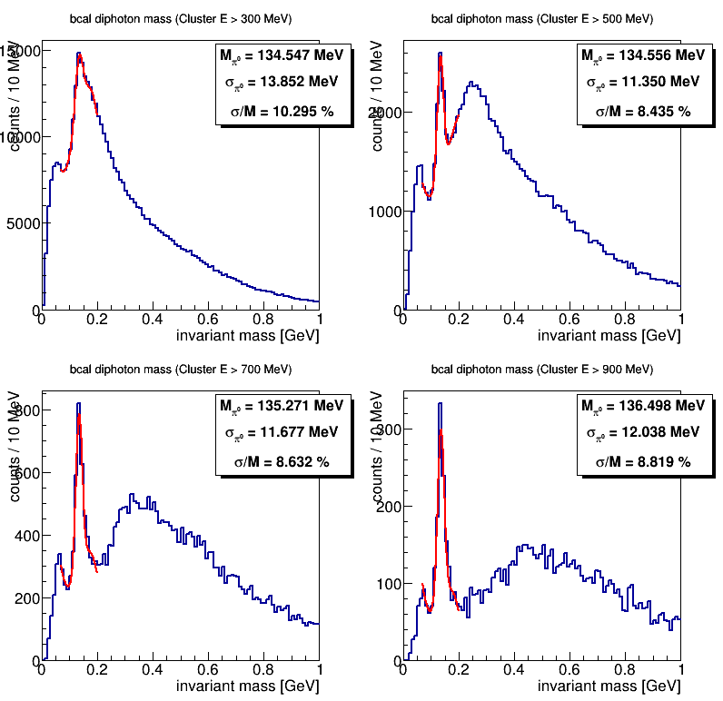
- Check BCAL pi0 - Reference: [ link ]
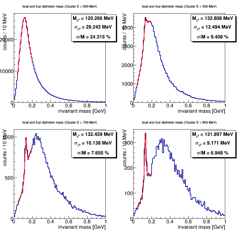
- Check BCAL/FCAL pi0 - Reference: [ link ]
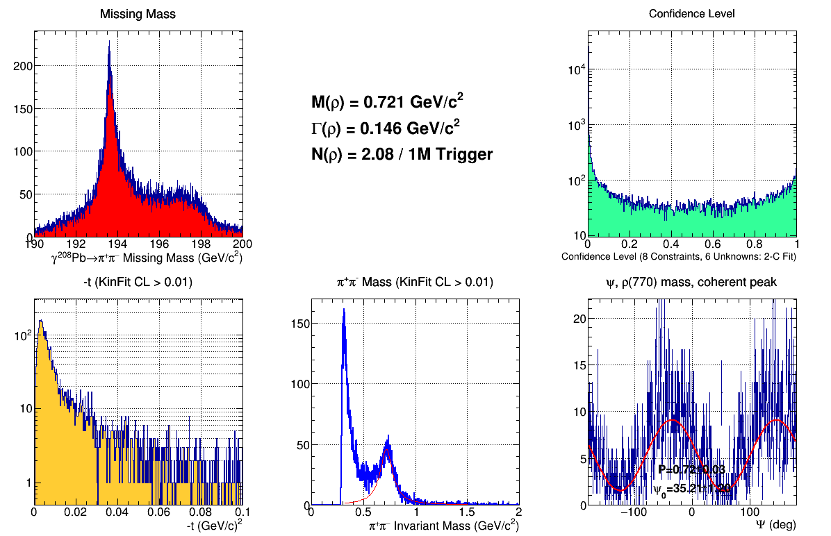
- Check CPP - Reference: [ link ]
Analysis Reference Plots
![]()
![]()
Analysis Notes
Generally in these plots, there will be a difference between diamond and amorphous radiator running. Should probably add some references for non-diamond plots.
- Tracking 1 - There should be some mild dependence on beam current and radiator. Note the spikes in the upper right plot are because we have 4 hypotheses fit to a track by default. The lower left plot does have a peak at zero.
- Tracking 3 -
- Check BCAL pi0 - The fitted peak should near at the correct pi0 mass of 135 MeV.
- Check BCAL/FCAL pi0 - The fitted peak should be lower than the correct pi0 mass, I think because the wrong vertex is used.
- Check CPP - The top left plot should have a peak at 193.5 GeV, the bottom middle plot a visible rho peak at 0.75GeV and the bottom right plot a sin(2phi) shape for diamond runs. Note that the yields in the center pad in the top row may vary significantly depending on the target.