Difference between revisions of "Offline Monitoring Data Validation CPP"
(→SC) |
(→SC) |
||
| Line 275: | Line 275: | ||
'''SC Notes''' | '''SC Notes''' | ||
| + | <div class="mw-collapsible-content"> | ||
| + | |||
| + | <html> | ||
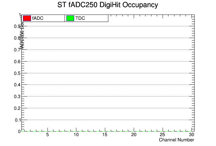
* ST Occupancy: The occupancies should be fairly even with some modulation vs. channel number. The TDC occupancy is expected to be higher than the fADC occupancy. | * ST Occupancy: The occupancies should be fairly even with some modulation vs. channel number. The TDC occupancy is expected to be higher than the fADC occupancy. | ||
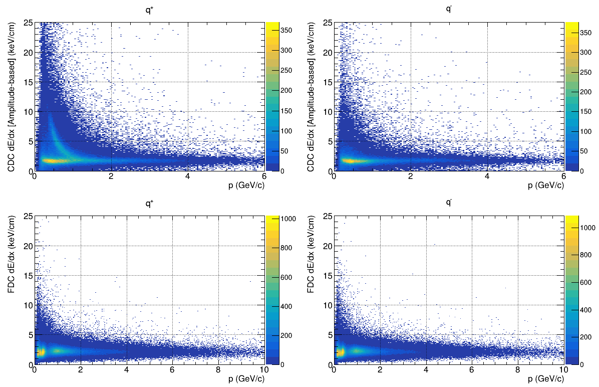
* ST Recon 1: There should be a clear separation between the proton and pion bands in the q+ dE/dx vs. p, and just a pion band in the corresponding q- distribution. | * ST Recon 1: There should be a clear separation between the proton and pion bands in the q+ dE/dx vs. p, and just a pion band in the corresponding q- distribution. | ||
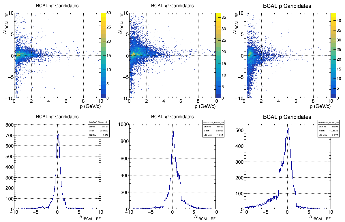
* ST Recon 2: The pi- and pi+ delta T distributions should be peaked near zero with a gaussian width < 1 ns. | * ST Recon 2: The pi- and pi+ delta T distributions should be peaked near zero with a gaussian width < 1 ns. | ||
* ST Matching: These plots are a little complicate, but the main thing is that the matching vs. track-z should be mostly above 90% | * ST Matching: These plots are a little complicate, but the main thing is that the matching vs. track-z should be mostly above 90% | ||
| − | |||
| − | |||
| − | |||
| − | |||
</html> | </html> | ||
Revision as of 16:09, 2 November 2023
This page contains the procedure for checking if CPP/NPP production runs are of good quality and can be used for physics analysis.
Contents
Procedure
For each production run, do the following:
- Go to the Offline Run Browser page.
- Follow the steps outlined in the checklist below.
- Workers should check each plot for their assigned subsystem and leave notes in the corresponding spreadsheet if any significant deviations are seen
- On the spreadsheet, enter "Y" in the "Overall Quality" field if all monitoring histograms are acceptable, otherwise enter "N"
- We will iterate this procedure until the process converges
Expert Actions
- Certify that each subsystem is okay
- Set run status in RCDB based on monitoring results
- (script provided)
Run Statuses
- -1 - unchecked
- 0 - rejected (not physics-quality)
- 1 - approved
- 2 - approved long/"mode 8" data
- 3 - calibration / systematic studies
Checklist
Reference run for 2022-05: 100987
General Notes
- Diamond and amorphous (AMO) runs have different beam energy spectra, which leads differences in reaction yields distributions which depend on the kinematics of the produced particles.
- The list of experts on different detector/calibration
BCAL
- Check Occupancy - Reference: [ link ]
- Check Hit Efficiency - Reference: [ link ]
- Check Recon. BCAL 1 - Reference: [ link ]
- Check Recon. BCAL 2 - Reference: [ link ]
- Check Recon. BCAL 3 - Reference: [ link ]
- Check BCAL Matching - Reference: [ link ]
BCAL Reference Plots


BCAL Notes
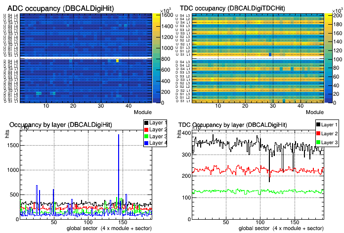
The BCAL is used to measure the energy and time of showers.
- Occupancy: This should be approximately flat. There can be hot channels when the baseline drifts. If we're running ask for a pedestal calibration to be done. If we're not running nothing can be done but a very hot channel might explain low efficiency in that area.
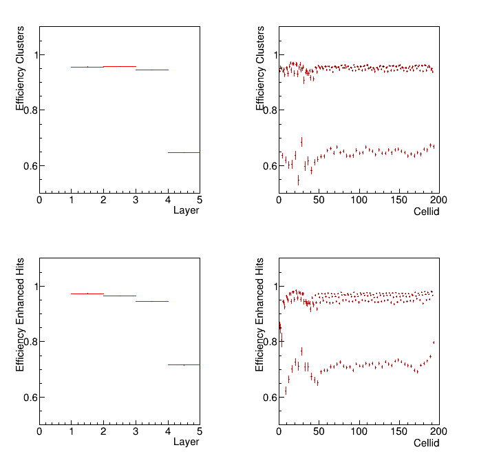
- Hit Efficiency: This should be approximately flat. If there are features we should understand why.
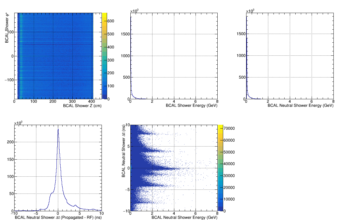
- Recon. BCAL 1: The histograms are somewhat complicated. The best is to compare them to a good run (the example above.) A difference from the example should be flagged.
- Recon. BCAL 2: The histograms are somewhat complicated. The best is to compare them to a good run (the example above.) A difference from the example should be flagged.
- Recon. BCAL 3: The histograms are somewhat complicated. The best is to compare them to a good run (the example above.) A difference from the example should be flagged.
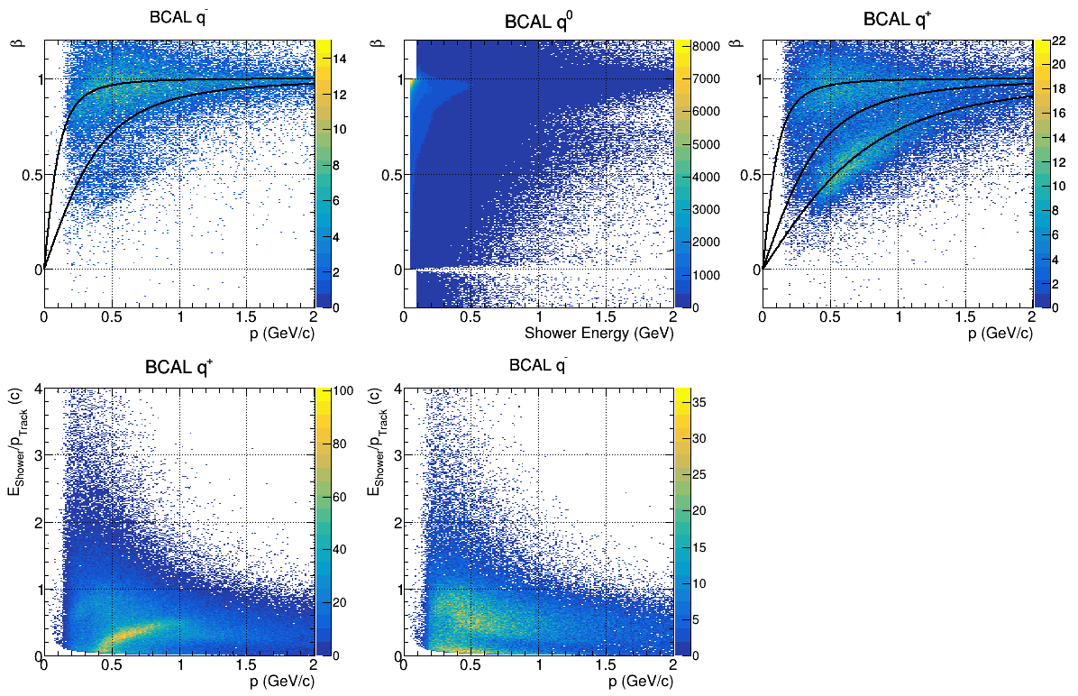
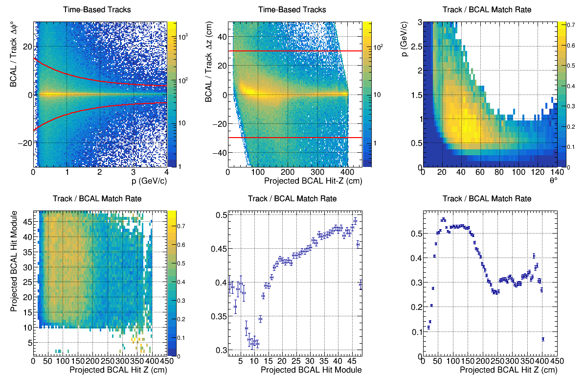
- BCAL Matching: These plots are for charged particles that are tracked in the drift chambers and projected to the BCAL. The z position along the BCAL can be calculated using the time difference between upstream and downstream hits and compared to the extrapolated position using the drift chambers. The histograms are somewhat complicated. The best is to compare them to a good run (the example above.) A difference from the example should be flagged.
- BCAL / Track Delta z (cm): (z determined from time of up - down hits in BCAL) - (z determined from the extrapolation of tracks in the drift chambers)
- projected BCAL Hit-Z (cm): z determined by extrapolating tracks in the drift chambers to the BCAL.
- Track / BCAL Match Rate: The match rate is the ratio of (number of hits in the BCAL that match the extrapolation of tracks in the drift chamber) / (number of tracks in the drift chamber that point at the BCAL).
CDC
- Check Occupancy - Reference: [ link ]
- Check Time-to-distance - Reference: [ link ]
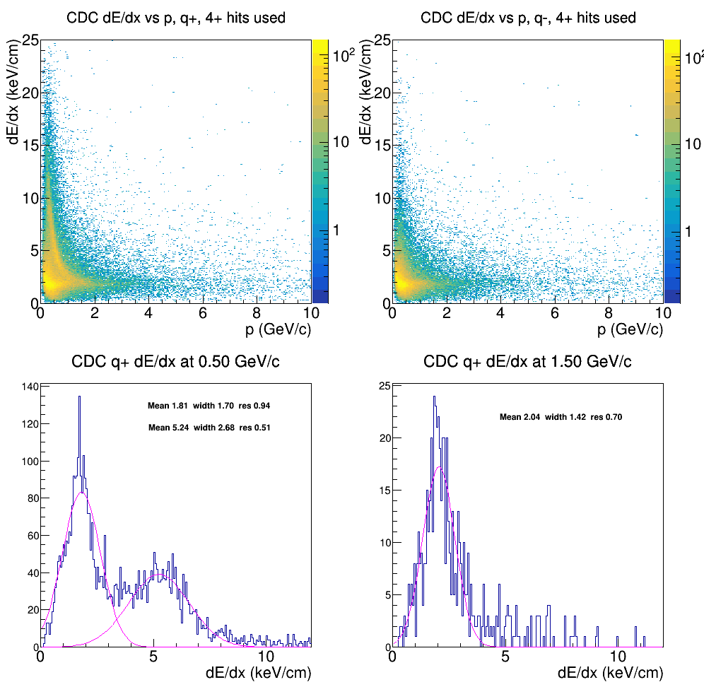
- Check dE/dx - Reference: [ link ]
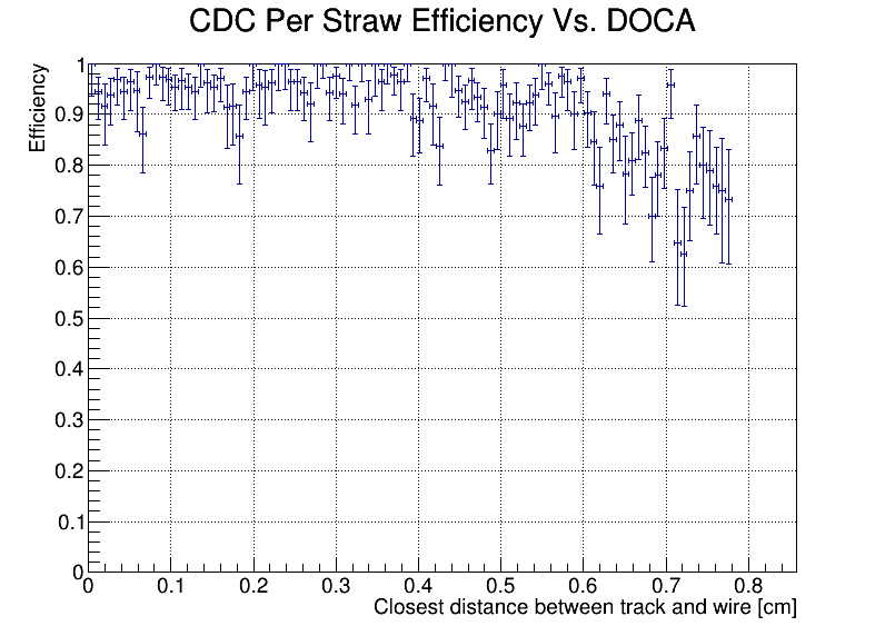
- Check Efficiency- Reference: [ link ]
CDC Reference Plots


CDC Notes
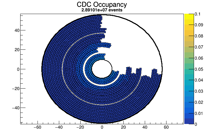
CDC Occupancy: There should be a uniform decrease in intensity from the center of the detector outward. Random white cells scattered throughout occur when not enough data were collected, eg empty target runs, trigger tests or no beam. Several contiguous white, dark blue or bright yellow cells which don't match the neighboring cells are a problem.
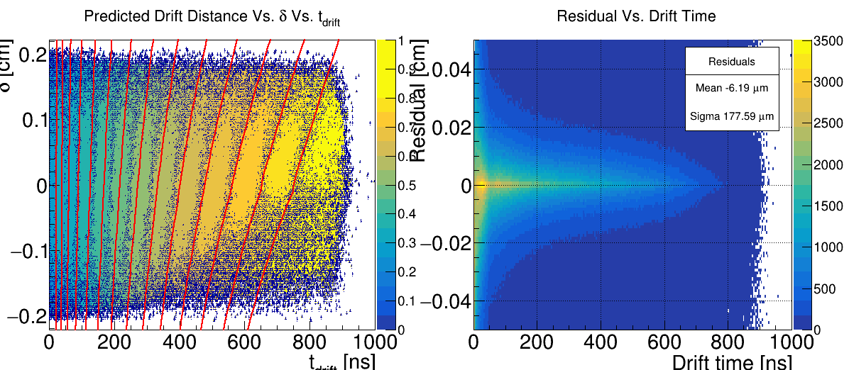
Time-to-distance: 𝛿, the change in length of the LOCA caused by the straw deformation, is
plotted against the measured drift time, t drift . The color scale indicates the distance of
closest approach between the track and the wire, obtained from the tracking software.
The red lines are contours of the time-to-distance function for constant drift distances
from 1.5 mm to 8 mm, in steps of 0.5 mm. They should lie over the top of the dark blue contour lines separating the colour blocks.
For the plot of residuals vs drift time, the mean should be less than 15um and the sigma should be less than 150um.
dE/dx: At 1.5GeV/c the fitted peak mean should be within 1% of 2.02 keV/cm.
Efficiency: The efficiency should be 0.98 or higher at 0cm DOCA, gradually fall to 0.97 at approximately 0.5mm and then more steeply through 0.9 at approximately 0.64cm.
FCAL
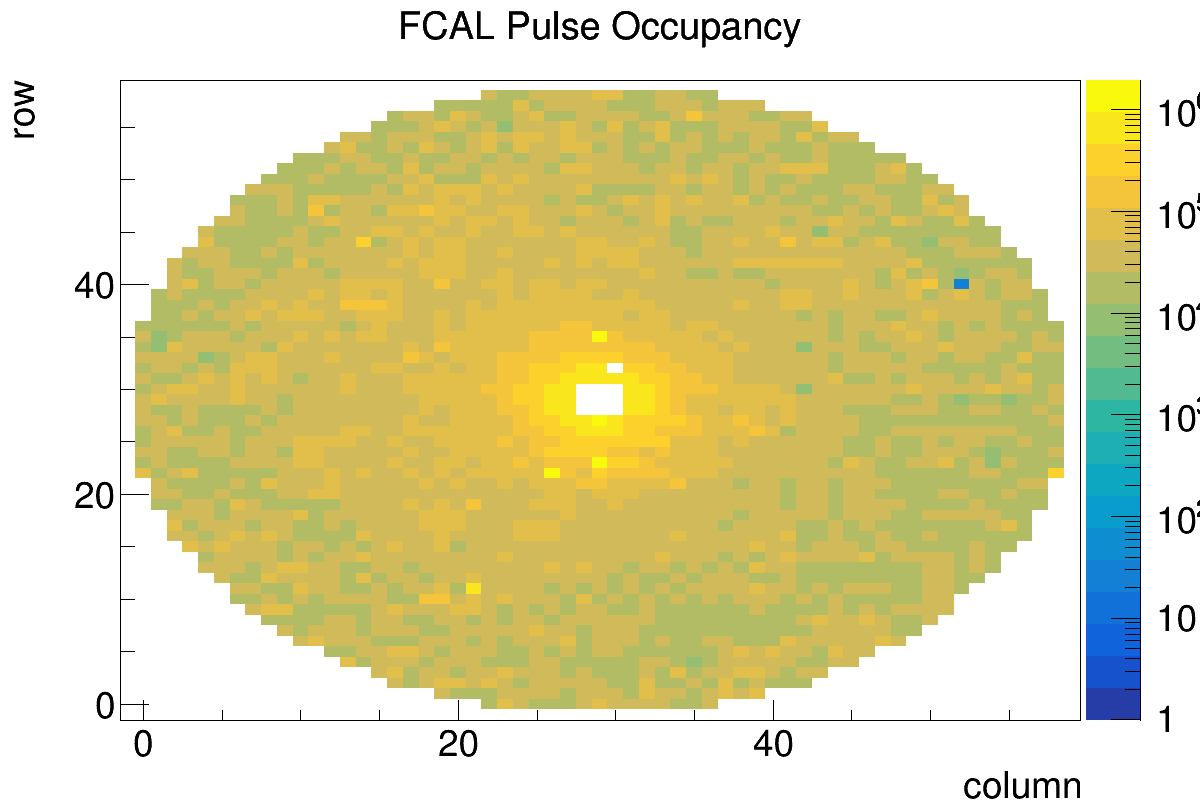
- Check Occupancy - Reference: [ link ]
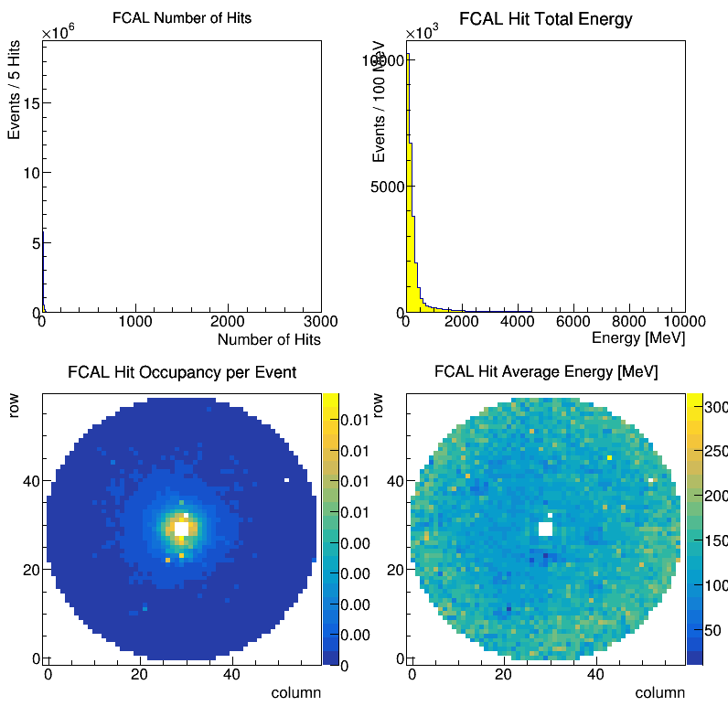
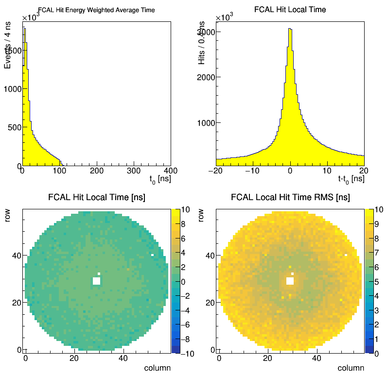
- Check FCAL Hits 1 - Reference: [ link ]
- Check FCAL Hits 2 - Reference: [ link ]
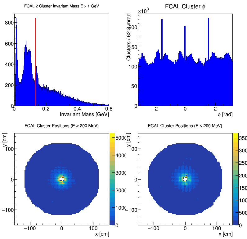
- Check FCAL Clusters 1 - Reference: [ link ]
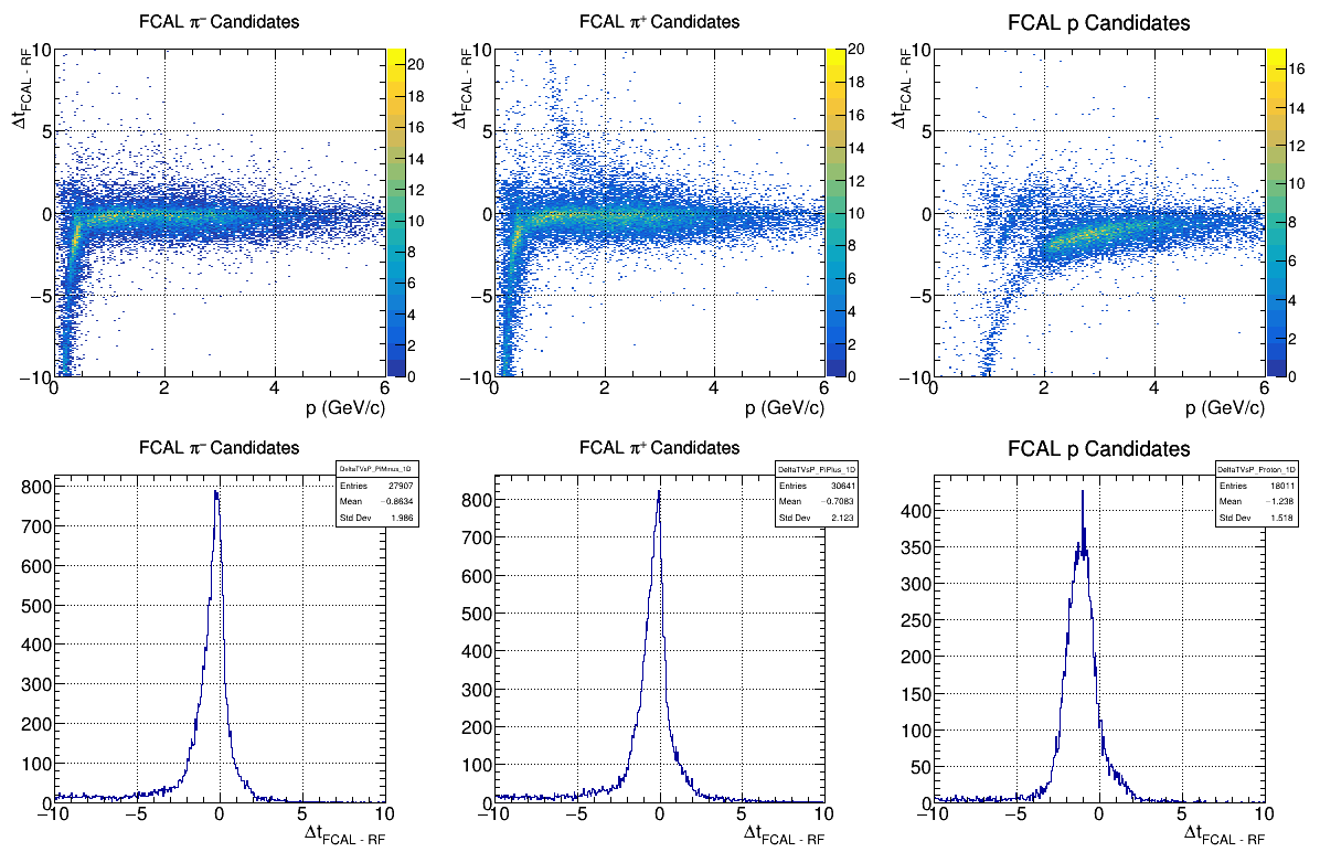
- Check FCAL Recon. 1 - Reference: [ link ]
- Check FCAL Recon. 2 - Reference: [ link ]
- Check Recon. FCAL Matching - Reference: [ link ]
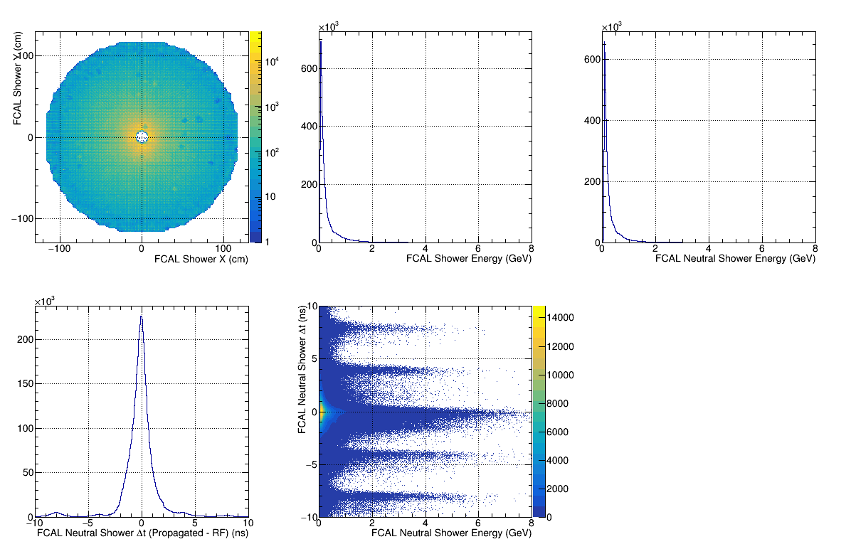
FCAL Reference Plots


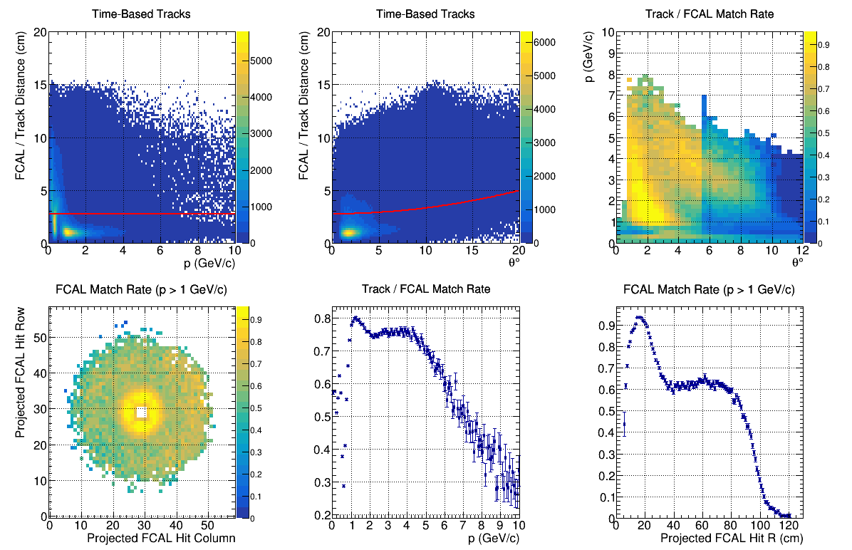
FCAL Notes
Is used for neutral particle detection and pion identification.
- Check Occupancy:
- Check FCAL Hits 1:
- Check FCAL Hits 2:
- Check FCAL Clusters 1:
- Check FCAL Recon. 1:
- Check FCAL Recon. 2:
- Check Recon. FCAL Matching:
FDC
- Check Package 1 Occupancy - Reference: [ link ]
- Check Package 2 Occupancy - Reference: [ link ]
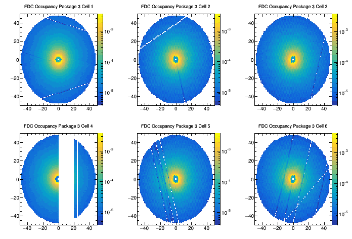
- Check Package 3 Occupancy - Reference: [ link ]
- Check Package 4 Occupancy - Reference: [ link ]
FDC Reference Plots
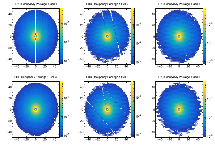
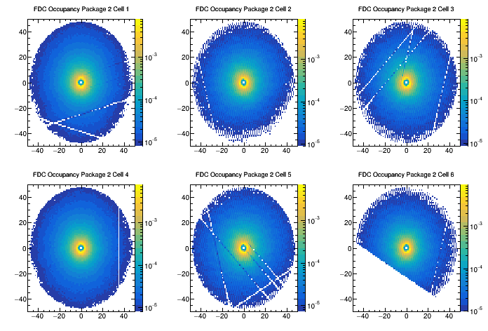

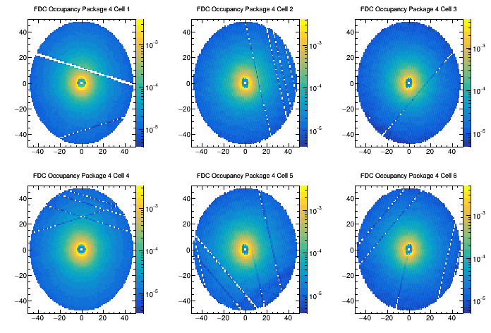
FDC Notes
PS
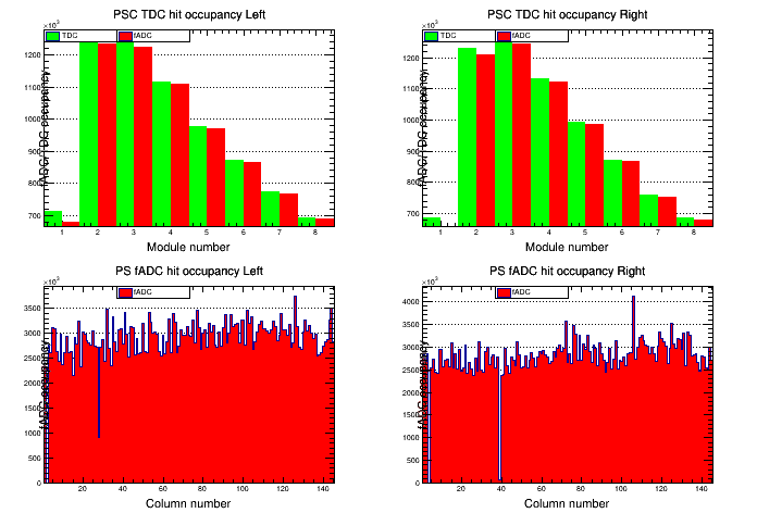
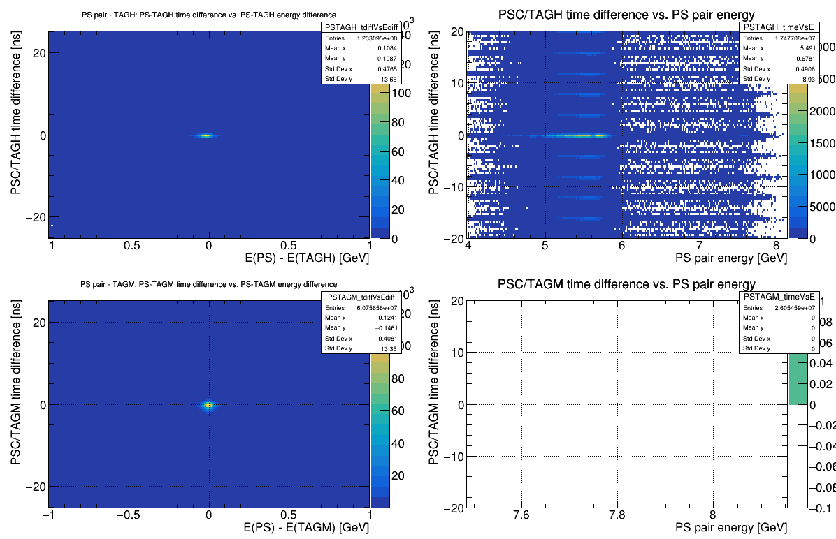
PS Reference Plots

PS Notes
SC
- Check Occupancy - Reference: [ link ]
- Check Recon. SC 1 - Reference: [ link ]
- Check Recon. SC 2 - Reference: [ link ]
- Check Recon. SC Matching - Reference: [ link ]
SC Reference Plots
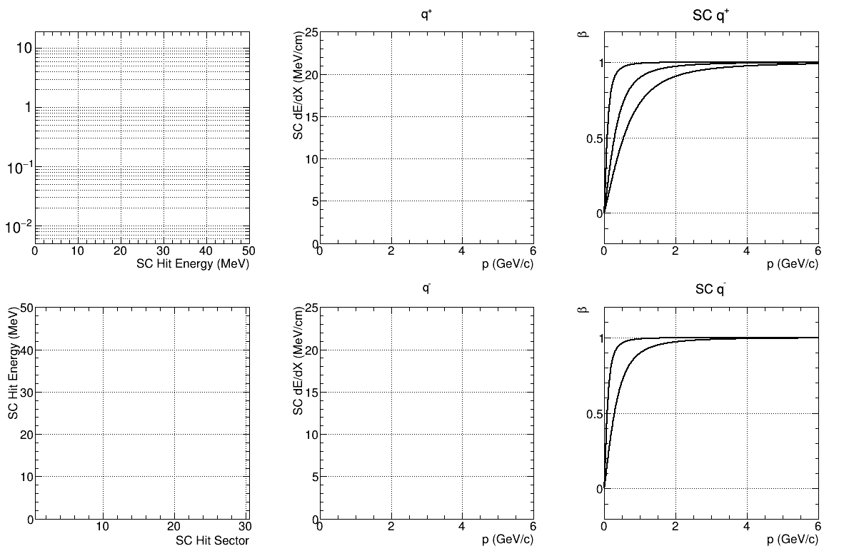
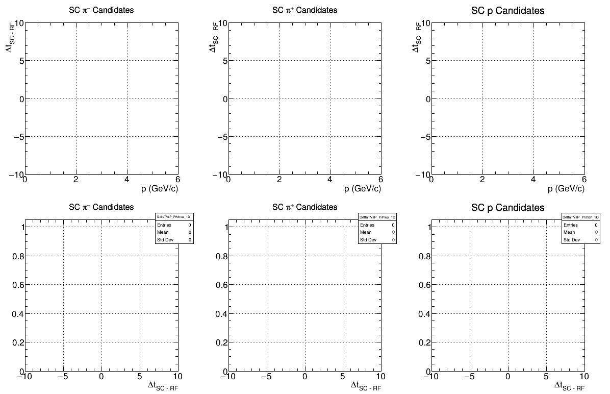
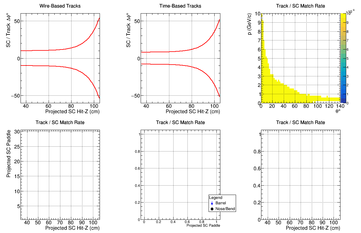
SC Notes
* ST Occupancy: The occupancies should be fairly even with some modulation vs. channel number. The TDC occupancy is expected to be higher than the fADC occupancy. * ST Recon 1: There should be a clear separation between the proton and pion bands in the q+ dE/dx vs. p, and just a pion band in the corresponding q- distribution. * ST Recon 2: The pi- and pi+ delta T distributions should be peaked near zero with a gaussian width < 1 ns. * ST Matching: These plots are a little complicate, but the main thing is that the matching vs. track-z should be mostly above 90%
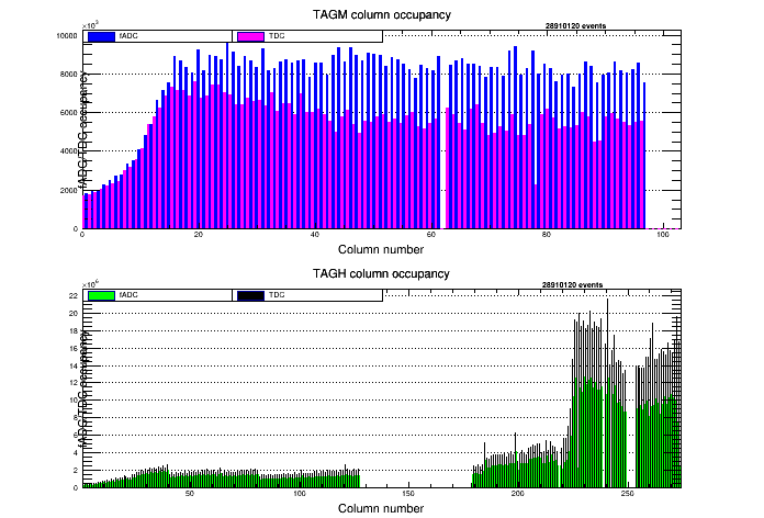
TAGH
TAGH Reference Plots

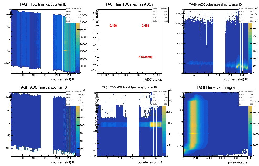
TAGH Notes
TAGM
TAGM Reference Plots

TAGM Notes
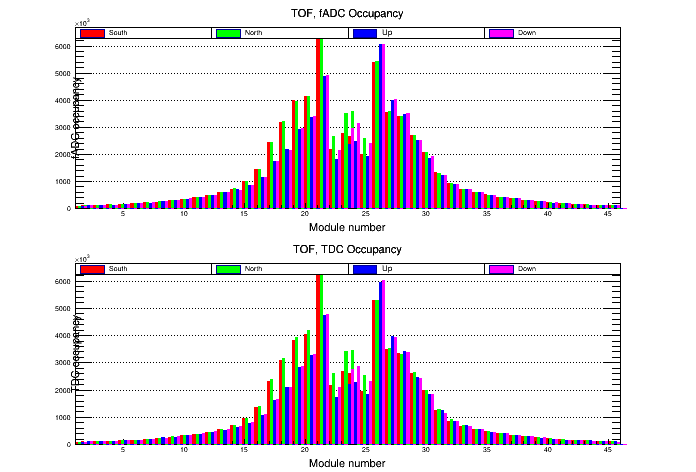
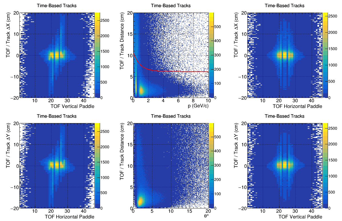
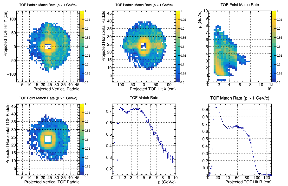
TOF
- Check Occupancy - Reference: [ link ]
- Check TOF Matching 1 - Reference: [ link ]
- Check TOF Matching 2 - Reference: [ link ]


TOF Notes
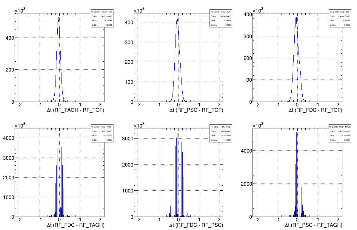
RF
- Check timing offsets - Reference: [ link ]
- Should be centered around zero
RF Reference Plots
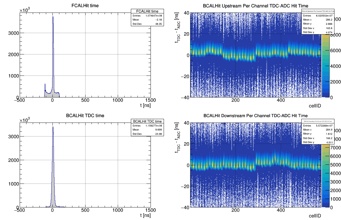
Timing
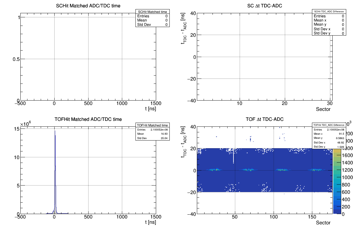
- Check HLDT Calorimeter Timing - Reference: [ link ]
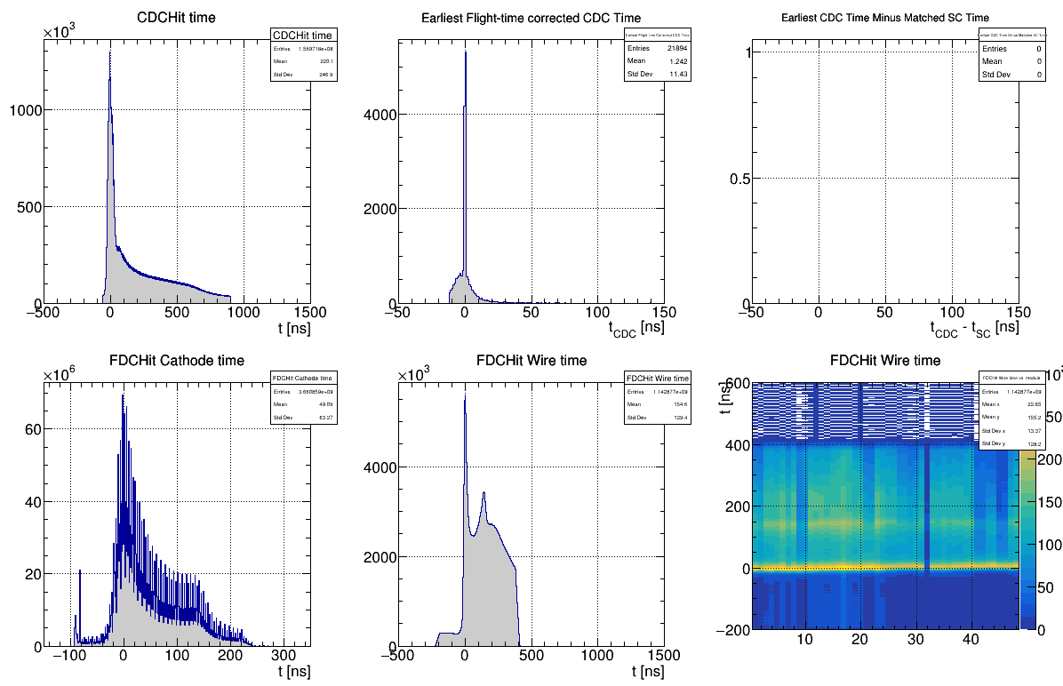
- Check HLDT Drift Chamber Timing - Reference: [ link ]
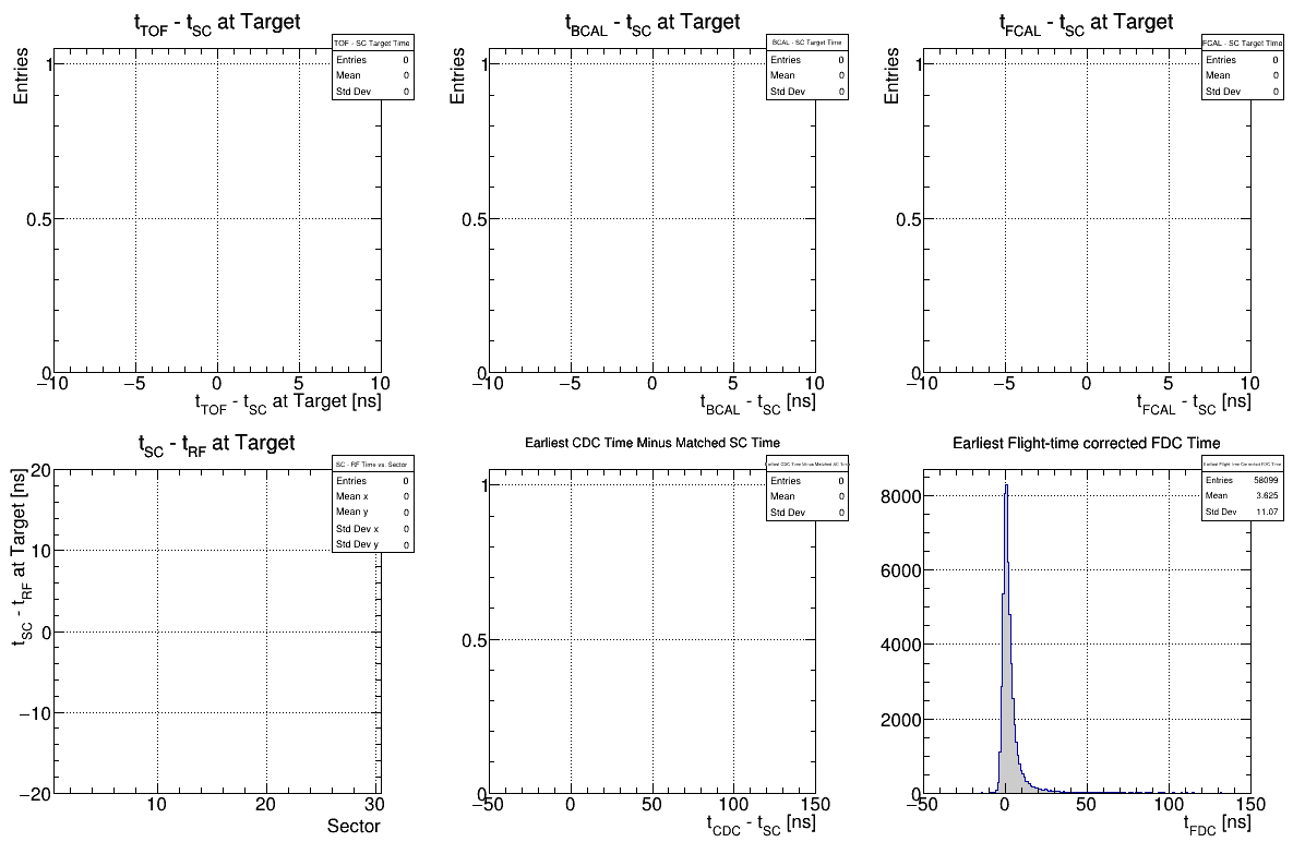
- Check HLDT PID System Timing - Reference: [ link ]
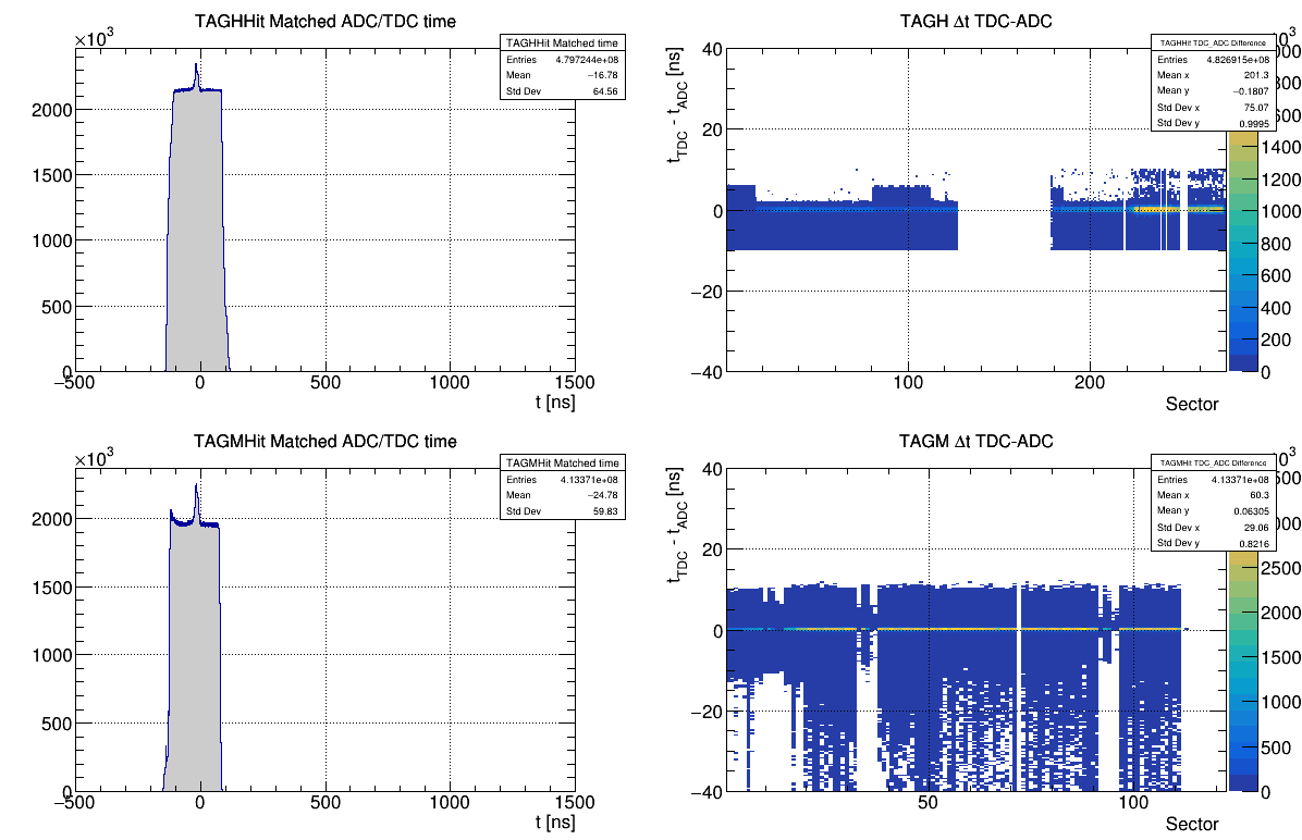
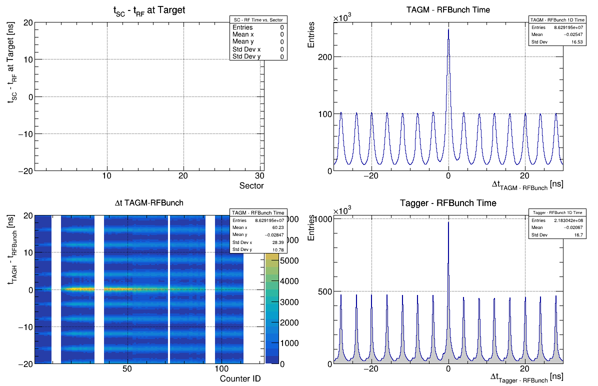
- Check HLDT Tagger Timing - Reference: [ link ]
- Check HLDT Tagger/RF Align 2 - Reference: [ link ]
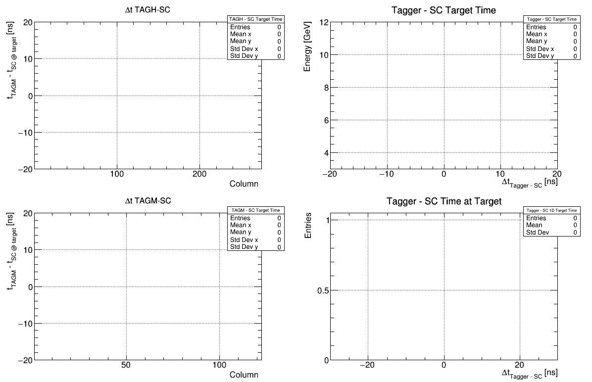
- Check HLDT Tagger/SC Align - Reference: [ link ]
- Check HLDT Track-Matched Timing - Reference: [ link ]
Timing Reference Plots

![]()


Timing Notes
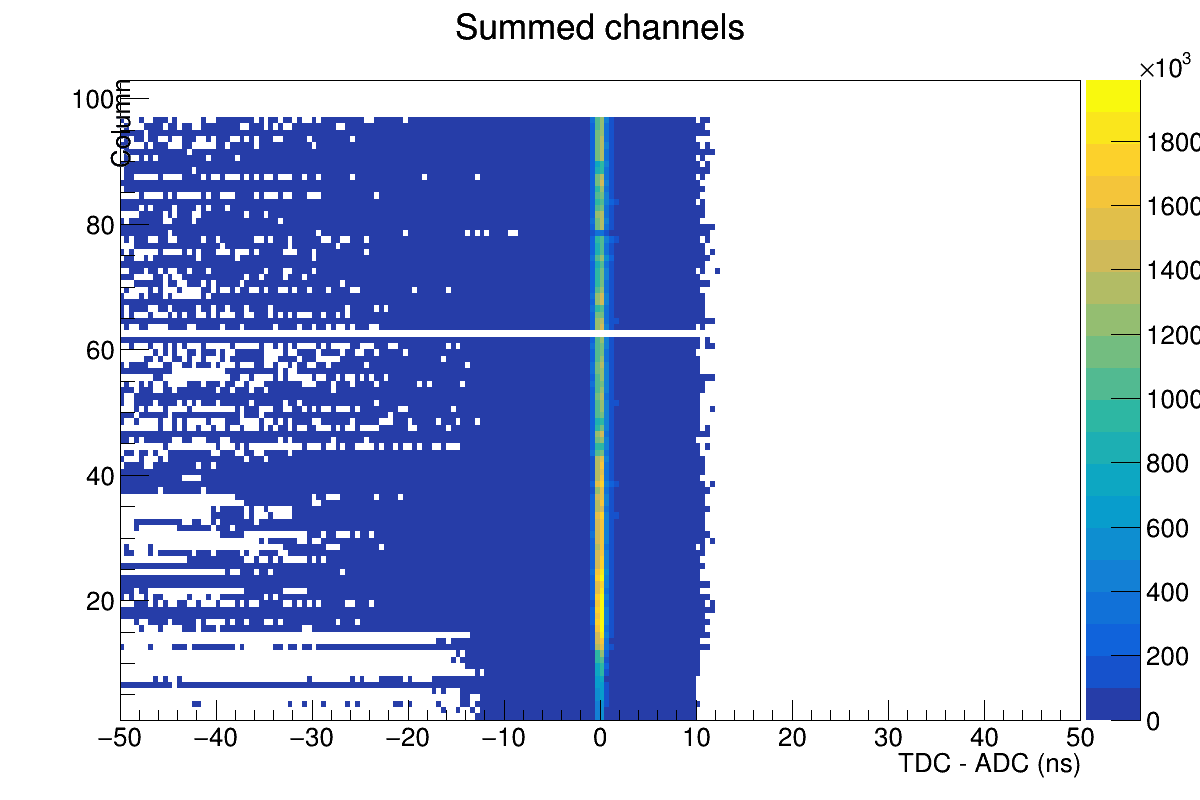
- Calorimeter Timing - The right two plots aren't aligned at zero because not all corrections are currently applied. If there is a 32 ns shift in part of this data, please note this.
- Drift Chamber Timing - In each case, the main peaks should line up at zero, but often have other structures. Ignore the first few bins of the lower left plot (they mostly say something about the noise in the detector). There can be 32 ns shifts in the lower right plot.
- PID System Timing - Nothing to note yet.
- Tagger Timing - The signal to background levels of the left two plots depend on the electron beam current.
- Track Matched Timing - Some overlap here with the tracking timing. The new plots should be centered at zero.
- Tagger/RF Timing - Look for the nice "picket fences" on the right two plots, and that in the bottom left plot each channel peaks at zero.
- Tagger/SC Timing - Should be similar to Tagger/RF Timing but with larger resolution.
Analysis
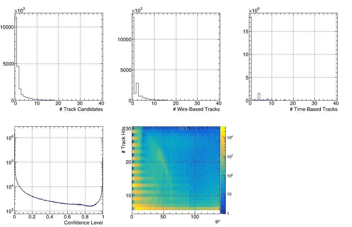
- Tracking 1 - [ link ]
- Tracking 3 - [ link ]
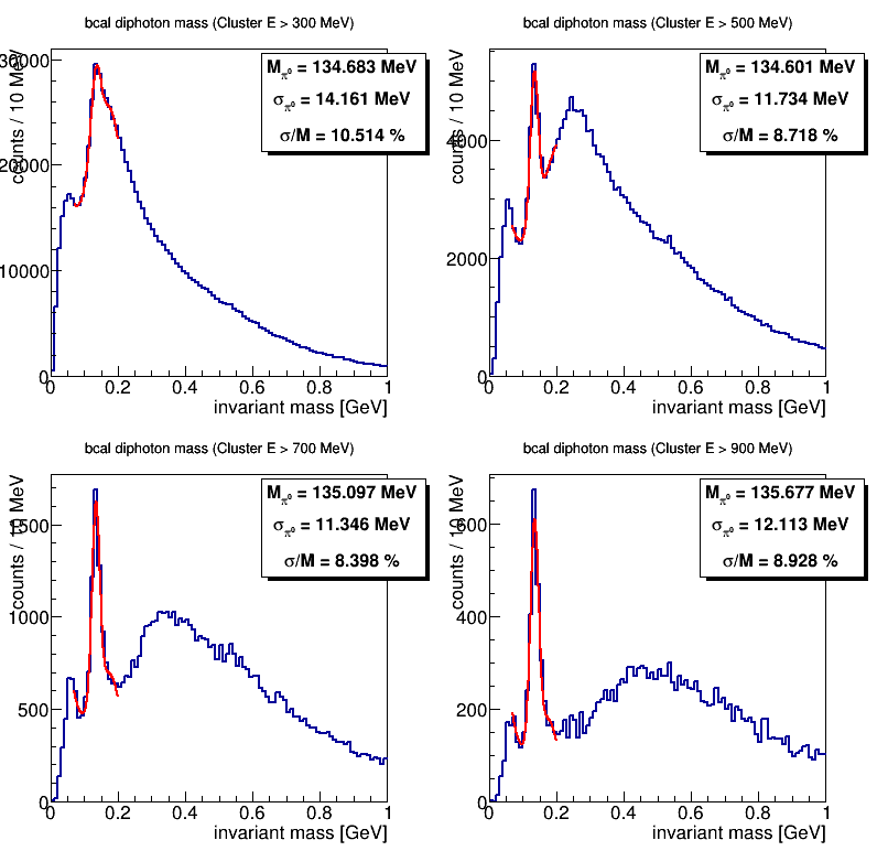
- Check BCAL pi0 - Reference: [ link ]
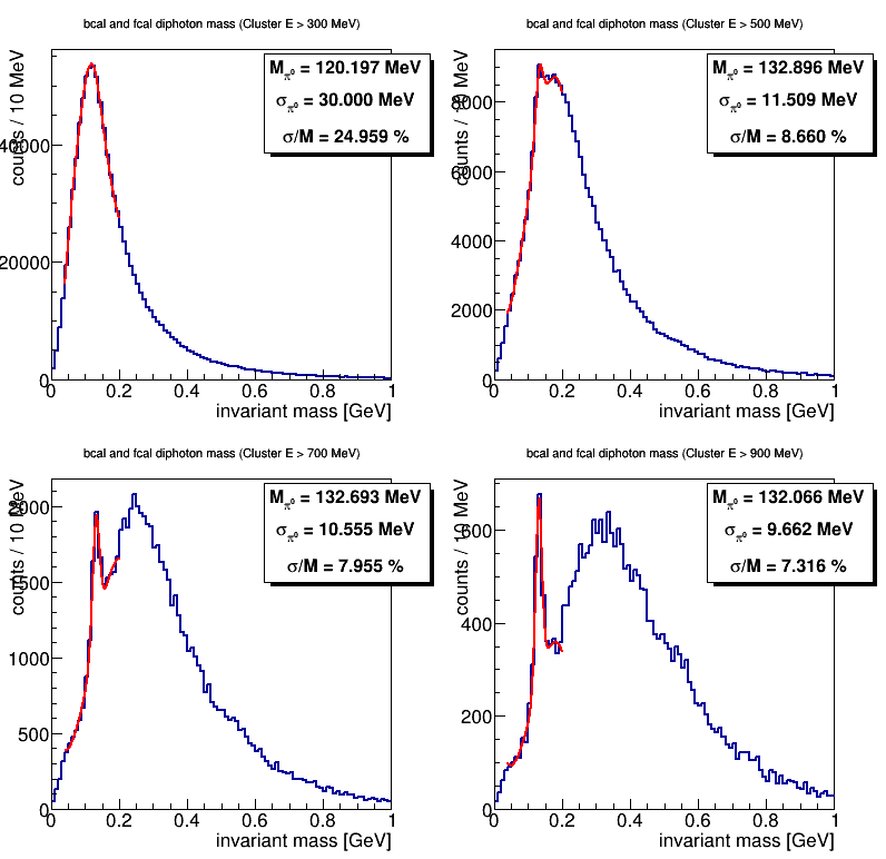
- Check BCAL/FCAL pi0 - Reference: [ link ]
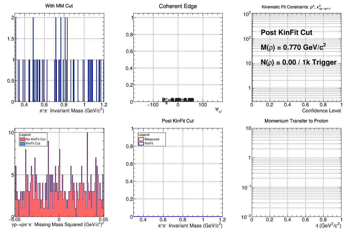
- Check p+2pi - Reference: [ link ]
- Check p+3pi - Reference: [ link ]
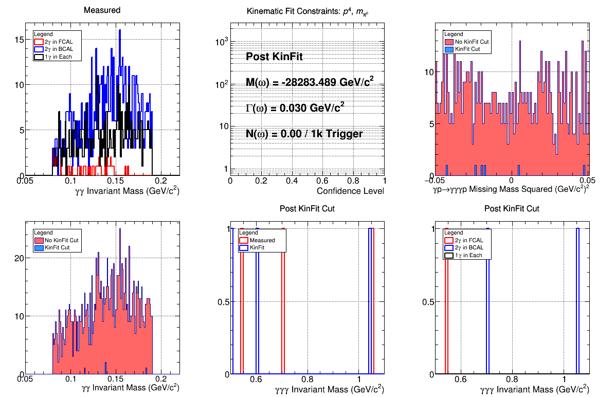
- Check p+pi0g - Reference: [ link ]
Analysis Reference Plots
![]()
![]()


Analysis Notes
Generally in these plots, there will be a difference between diamond and amorphous radiator running. Should probably add some references for non-diamond plots.
- Tracking 1 - There should be some mild dependence on beam current and radiator. Note the spikes in the upper right plot are because we have 4 hypotheses fit to a track by default. The lower left plot does have a peak at zero.
- Tracking 3 -
- Check BCAL pi0 - The fitted peak should near at the correct pi0 mass of 135 MeV.
- Check BCAL/FCAL pi0 - The fitted peak should be lower than the correct pi0 mass, I think because the wrong vertex is used.
- Check p+2pi - The top middle plot should have a sin(2phi) shape for diamond runs. Note that the yields in the top right plot vary from run to run on the order of 10-20%.
- Check p+3pi -Note that the yields in the top right plot vary from run to run on the order of 10-20%.
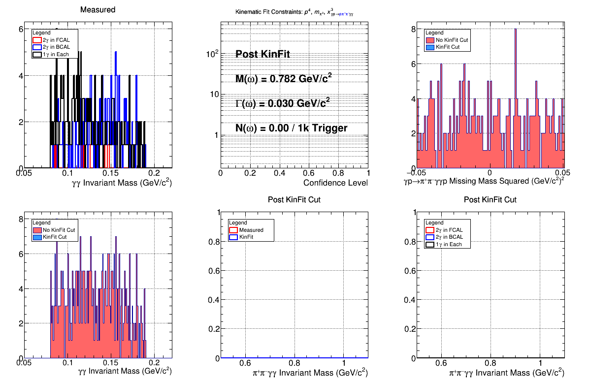
- Check p+pi0g - Note that the yields in the top right plot vary from run to run on the order of 10-20%.
- Note that these yields are sensitive to the tagger range used! This changes for different beam current settings.